
In the previous post, we talked about ways to tessellate a triangle with adaptive tess factors. Now it’s time to take the next step and actually tessellate a mesh. The goal of this post is to put together a reference solution, a baseline approach that works everywhere.
Here you can open the live WebGPU tessellation viewer. Or if you prefer you can download the viewer as a standalone zip. The code is MIT licensed so feel free to use it.
We’re going to use vanilla WebGPU (no extensions) with the intention to be scalable to mobile. There are numerous ways it could be improved (mesh shaders!) but we’ll make do with what we have.
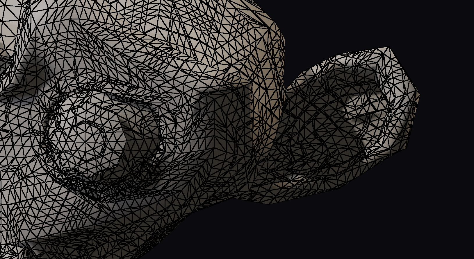
The algorithm is similar in spirit to Dx11 tessellation but we are making some decisions differently [4]. We’re going to be tessellating edges, choosing barycentrics, and then interpolating with Phong Tessellation [3]. So how do we actually do this with compute shaders?
The 1/16th Rule
There is an inherent tradeoff in tessellation. On one hand, we can create a very complex algorithm to figure out exactly how much each triangle should be tessellated. Or alternatively we can use a simple algorithm, and just brute force as many triangles as possible.
My rule of thumb is that each subdivision level is about 1/16th as efficient as the previous one. As tessellation levels increase, the value of each marginal triangle quickly falls off a cliff, which is why I value adaptation despite the cost. This is an opinion, not a fact. You do you.
In the 2d case, suppose we have a circle that we want to render. However, we can only render lines, so the simplest approach would be to start with a square and subdivide it. Here are a few subdivision levels. We can see that it converges quite well.
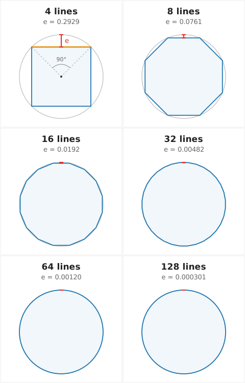
Each of those subdivision levels doubles the number of lines from the previous one. But more importantly, it converges very quickly.
| Level | Lines | Chord angle θ | Error e = 1 − cos(θ/2) | Reduction vs. prev |
|---|---|---|---|---|
| 0 | 4 | 90° | 0.2929 | — |
| 1 | 8 | 45° | 0.0761 | 3.85× |
| 2 | 16 | 22.5° | 0.0192 | 3.96× |
| 3 | 32 | 11.25° | 0.00482 | 3.99× |
| 4 | 64 | 5.625° | 0.00120 | 4.00× |
| 5 | 128 | 2.8125° | 0.000301 | 4.00× |
Looking at the table, each subdivision has 1/4th as much impact as the previous one. This behavior is similar to endpoint/trapezoid integration in calculus where doubling the number of samples causes a 4x reduction in error. Qualitatively, the impact from 0 to 1 is enormous but 4 looks indistinguishable from 5.
So in addition to paying 2x more for each level, we are also gaining 1/4x the quality improvement each time. Combined, that makes each level 1/8th as efficient as the previous one.
Turning to the 3d case, the same process holds, except that each subdivision costs us 4x the number of triangles, not 2x.
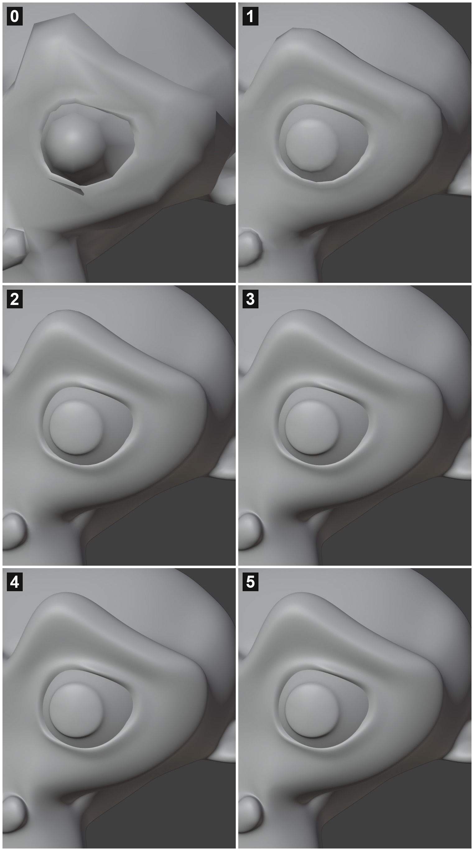
Catmull-Clark subdivision of Suzanne in Blender, levels 0-5 (one eye).
Computer graphics is all about tradeoffs, and for every cycle that we spend, we need to think about the opportunity cost of using that cycle somewhere else. The first few levels of subdivision provide a tremendous improvement at minimal cost. The last subdivision has very high cost but zero value (I wouldn’t be able to tell if they were flipped). And even if we could afford levels like 2 and 3, we would have to seriously consider if those cycles are better spent on lighting, shading, or something else.
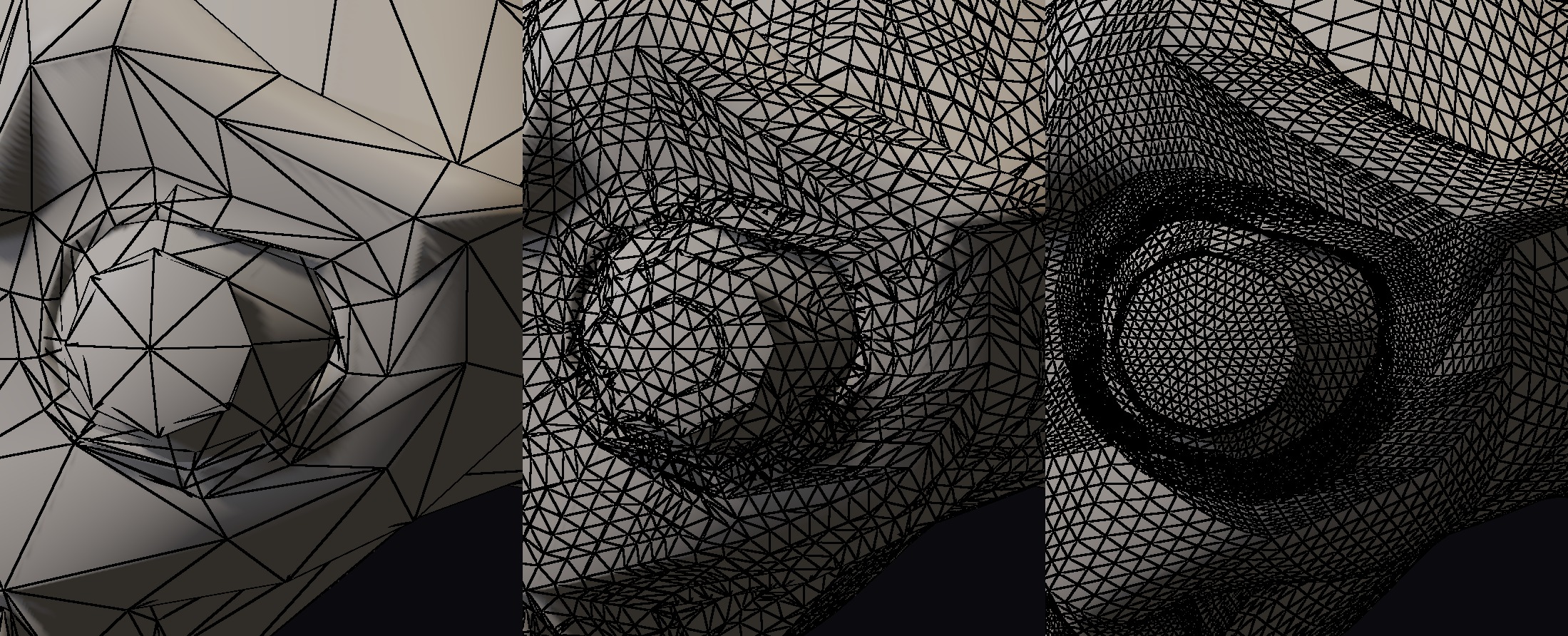
Let’s take a closer look at Suzanne, using a close-up view. Here are three variations of the same camera angle. The first with fixed tessellation, the second with adaptive tessellation at a similar triangle count, and the third image where I bumped up the tessellation until the quality was approximately at parity with adaptive.
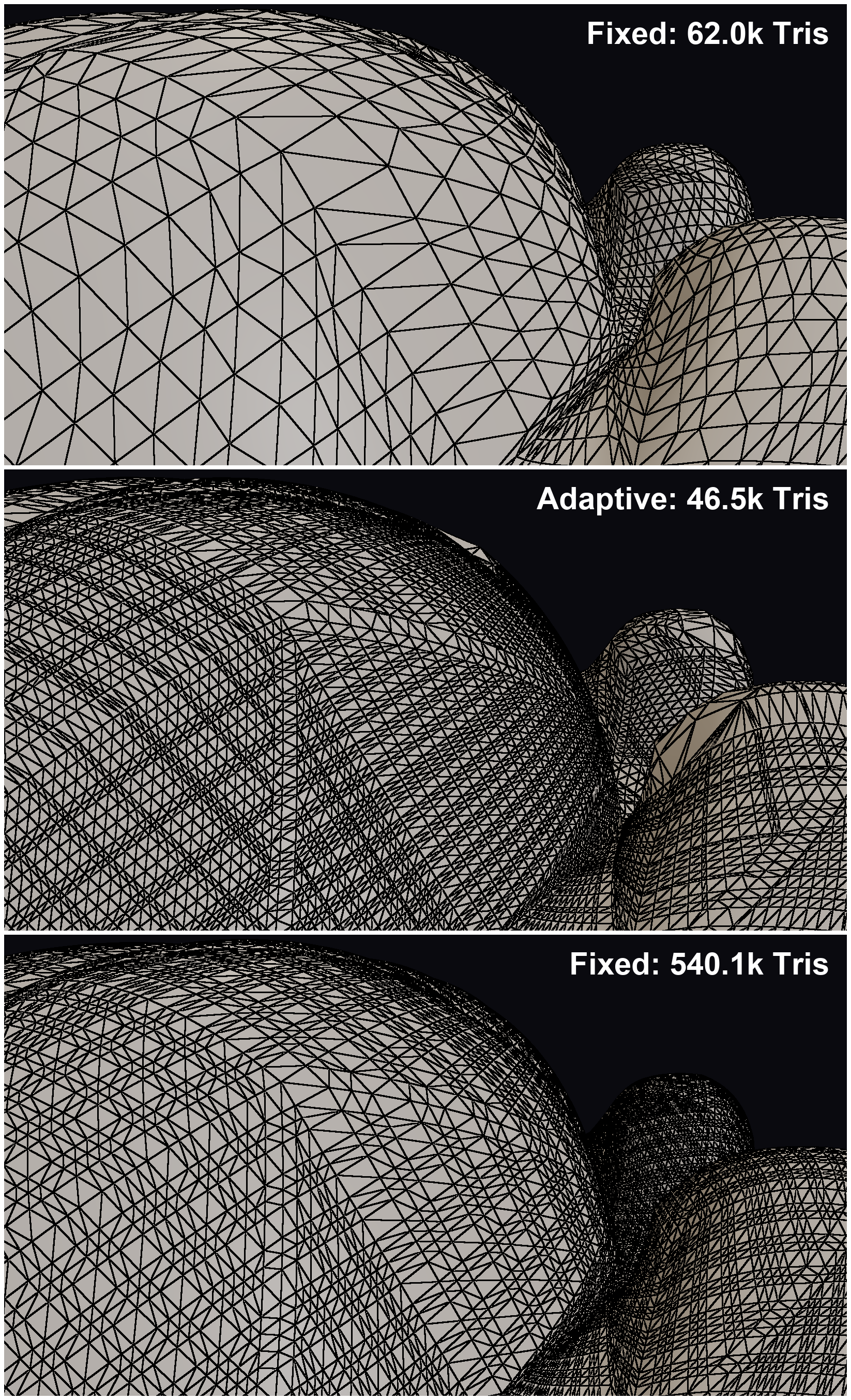
Adaptive vs. fixed-rate tessellation on Suzanne.
Certainly, it’s imperfect. The screen-space algorithm could use some tweaking. There are numerous variables in the construction of the model (organic vs manufactured meshes), the view angle, and the adaptivity metric. But the overall trend is clear: If we want to render large, immersive worlds on a wide range of devices, we’re going to need adaptive tessellation.
Welding Edges
If you have subdivision, what do you do about seams? For example, Suzanne has a UV seam along the middle, so if we naively displace the surface, we will have different values on either side causing cracks. This problem actually becomes quite complicated, as there are many reasons why seams might not line up, ranked from easiest to hardest to fix.
- Edge invariance: With float precision, in general, there is no guarantee that t=1-(1-t). There is more precision between, say, [0.25,0.5) than [0.5,1.0f). So if t < 0.5, and we calculate 1-t, we will lose precision. This issue pops up in B-splines and PN tessellation. Fortunately, this one is easy to fix if we are aware of it.
- Partial derivatives: If we want to use mipmapping for displacement (which we do!), then we will need to calculate the partial derivative analytically. And if we have to match the same partial derivative along the seam to guarantee the same displacement.
- Seams: Now things start getting tricky. Where we have a UV seam, we need the same value along both sides of the seam. One option is to smooth to zero, or another option is a special exception in the shader to ensure we use the same side for both positions. Both are burdensome for artists.
- Materials: What if we have a brick wall attached to a concrete floor? It’s theoreticaly possible if we have an ubershader, but if we have separate PSOs then I’m at loss for this one.
We need a general solution, and that means we need to weld edges. Fortunately, it’s realatively inexpensive to average the edge positions directly.
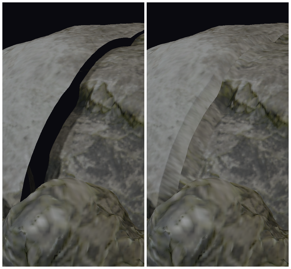
Without welding (left), the UV seam splits into a crack under displacement; welding the edges (right) closes it.
Stored Buffers
This leads to the first major design change from hardware tessellation. In hardware tessellation, each source triangle is independent. A triangle is input, generates a tessellation, and that tessellation is consumed. This makes the algorithm general, but makes it impossible to weld vertices afterwards. Instead, we are going to store the actual positions in a separate buffer that we calculate ahead of time. Then we can weld them manually before rasterizing them.
The downside is that we need to store the vertices in a giant buffer. This is fine. In general, meshes need to be rendered multiple times per frame (depth prep-pass, GBuffer/VBuffer, motion vectors, shadows), so it can actually be a win if the displacement function is expensive.
In theory, Dx11 hardware tessellation [4] has the advantage that triangles are consumed as they are produced, creating an elegant method of expansion while never needing to store the fully tessellated data. In reality, GPUs need to perform gymnastics to make this work, often involving roundtrips through VRAM. Additionally, if you have 5 passes with tessellation, then you have to calculate the same value 5 different times. But even if it was faster to generate vertices on-the-fly, the inability to weld is a fundamental limitation that we need to address.
The solution is a dedicated pass to write the triangles, and a dedicated pass to write the vertices. The vertices can be thin, storing the position, normal, and barycentric of the vertex. To be clear, the extra memory cost still hurts, but I’ll take that over the consequences of not having it.
This creates one more detail: How do we handle too many tessellated triangles overflowing our buffer? Since all tess factors are calculated at once, we know exactly how many triangles/vertices are required. This design allows us to check up front and change the tess factors as necessary. The current demo simply sets all tess factors to zero if we go over, but we could easily fail more gracefully.
Optimized Clamped Parallelogram Tessellation
In the previous post, the tessellation algorithm was split between a clamped parallelogram and a filled gap. After some testing, I found it was faster to create a lookup table for the clamped parallelogram section. It only depends on the pair of edges, and pre-building the full pattern and a lookup for the barycentrics is surprisingly reasonable. So at the very beginning, the app creates this lookup table of the index list and barycentric values up to a tess factor of 255, although we could reduce it.
| Max tess factor | Tokens | Total blob |
|---|---|---|
| 15 | 9 | 0.35 MB |
| 31 | 13 | 0.78 MB |
| 63 | 17 | 2.46 MB |
| 127 | 21 | 8.65 MB |
| 255 | 25 | 28.80 MB |
Tess Factors
Given the actual edges in the scene, how should we calculate tess factors? I have a general rule against using the actual screen-space length after the projection matrix, because I find that it’s a bit finicky and unstable. As a sanity test, if you simply spin the camera in a circle, the tess factors should stay the same (since it’s the same distance to the camera). So I prefer to calculate the angular arc length from the camera and convert that to a rough proxy in terms of pixels.
I really like Wade Brainerd’s approach from Call of Duty: Ghosts [1], as the distance from the midpoint of the line segment to the middle of the curve works well. Another approach is Nanite’s technique [2] which uses a modification of the screen-space distance. Ultimately I used angular edge length for this demo, but I plan to continue investigating once I have more relevant data sets.
Reverse Lookup
For each tessellated vertex, we need the ability to find which source triangle it came from. We could store this as a single int per vertex. But we can instead use the same prefix sum with bitmask trick that we used for matching. For each group of 32 output vertices, we store the start source vertex as well as a 32 bit mask if this bit increments the source triangle. This technique allows us to perform a fast O(1) reverse lookup with 2 bits per output vertex.
Compute Passes
The pipeline takes a source mesh and per-edge tess factors. It produces welded vertices containing a position, normal, and barycentric. All other attributes are interpolated in the VS. The triangle index buffer is ready to be consumed by the rasterizer. Note that this cost would be a nonstarter if we had to perform all these passes for every mesh. However, we can merge all meshes together so it becomes 14 passes total regardless of how many meshes we have. The one exception is the vertex displacement pass which needs to be unique for each displacement shader.
predict_tri: For each source triangle, predict how many output verts and tris its tess factors will produce.predict_cluster: Prefix sum for each cluster (verts, tris).offsets_cluster: Prefix sum the cluster totals to get each cluster's slice base in the pool.offsets_tri_cluster: Scan each tri for offset within cluster.offsets_tri_inst: Flat scan for every instance across every source tri, generating per-tri offset inside the whole instance.plan_wg_count: Prefix sum per cluster workgroup for total workgroup count.plan_wg_layout: Write per-workgroup metadata (which cluster, which prim range, srcTri-hint for cheap entry).patch_tri: Pack triangle information into packed 32-byte structs to minimize fetches later.patch_corners: Pack the triangle info for welding later.lookup_vert: Generate the O(1) reverse lookup.emit_indices: Output the actual triangle indices.emit_verts: Output the position/normal/barycentric for each tessellated vertex.weld_verts: Average position/normal across corner verts.weld_edges: Average position/normal across edge verts.
Discussion
In the spirit of testing for a wide range of devices, I’m capturing these numbers on my 7-year-old laptop with a GTX 1050. But since this is on WebGPU, feel free to capture numbers yourself.
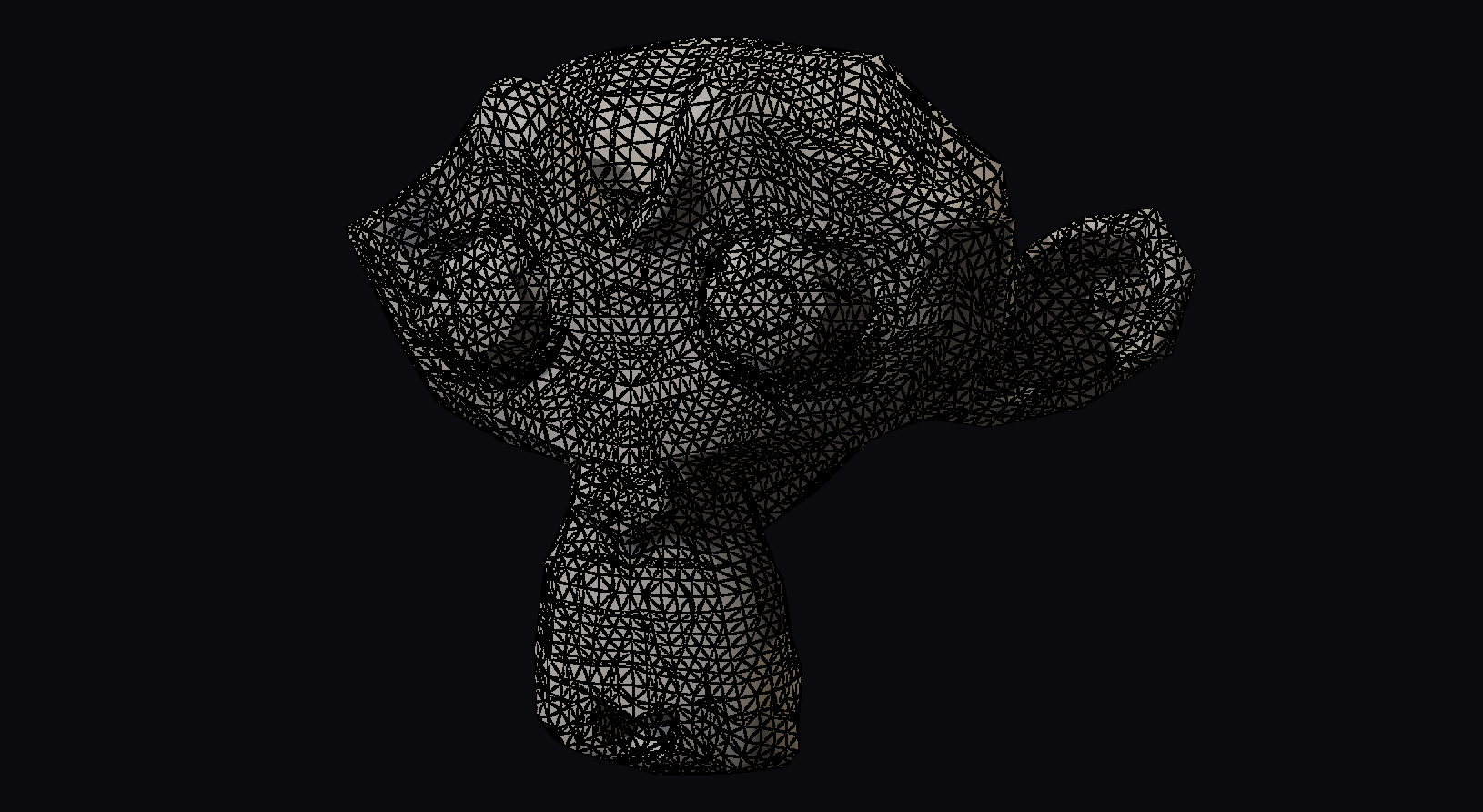
The shared camera angle for the five timing captures below (edge-angular adaptive tessellation shown).
Per-frame breakdown
| Metric | Adaptive | Fixed 0 | Fixed 15 | Fixed 31 | Fixed 127 |
|---|---|---|---|---|---|
| Mode | edge_angular | fixed | fixed | fixed | fixed |
| Tess factor | N/A | 0.0 | 15.0 | 31.0 | 127.0 |
| Tris | 23,560 | 968 | 247,808 | 995,104 | 15,886,816 |
| Verts | 19,785 | 2,904 | 148,104 | 544,984 | 8,130,232 |
| Tessellation (ms) | 0.458 | 0.336 | 0.453 | 1.037 | 14.805 |
| Render (ms) | 1.494 | 1.442 | 0.958 | 1.410 | 16.863 |
| Shadow light 0 (ms) | 0.089 | 0.022 | 0.229 | 0.920 | 16.441 |
| Shadow light 1 (ms) | 0.071 | 0.016 | 0.188 | 0.700 | 12.406 |
| Shadow light 2 (ms) | 0.087 | 0.023 | 0.245 | 0.948 | 16.782 |
| Shadow light 3 (ms) | 0.065 | 0.018 | 0.208 | 0.780 | 13.660 |
| Wire overlay (ms) | 0.157 | 0.059 | 0.378 | 1.321 | 22.243 |
Tessellation passes (ms)
| Tessellation pass | Adaptive | Fixed 0 | Fixed 15 | Fixed 31 | Fixed 127 |
|---|---|---|---|---|---|
predict_tri |
0.026 | 0.020 | 0.011 | 0.011 | 0.012 |
predict_cluster |
0.026 | 0.024 | 0.012 | 0.011 | 0.013 |
offsets_cluster |
0.012 | 0.013 | 0.006 | 0.006 | 0.005 |
plan_wg_count |
0.010 | 0.016 | 0.006 | 0.006 | 0.018 |
plan_wg_layout |
0.031 | 0.024 | 0.014 | 0.014 | 0.033 |
patch_tri |
0.025 | 0.020 | 0.011 | 0.011 | 0.011 |
emit_indices |
0.099 | 0.063 | 0.144 | 0.424 | 7.206 |
lookup_vert |
0.038 | 0.032 | 0.026 | 0.048 | 0.500 |
patch_corners |
0.036 | 0.034 | 0.016 | 0.014 | 0.014 |
offsets_tri_cluster |
0.017 | 0.014 | 0.008 | 0.007 | 0.006 |
offsets_tri_inst |
0.015 | 0.014 | 0.008 | 0.007 | 0.005 |
emit_verts |
0.084 | 0.034 | 0.169 | 0.459 | 6.950 |
weld_verts |
0.016 | 0.015 | 0.009 | 0.007 | 0.006 |
weld_edges |
0.023 | 0.011 | 0.010 | 0.010 | 0.025 |
Observations:
- For higher tessellation levels, the full cost of pre-computation is roughly the same or a little more than the direct shadow render passes.
- At a glance, the cost seems reasonable. Spending less than 1ms for higher quality characters and hero assets seems plausible on low-end PC and mid/high spec mobile hardware.
- The minimum cost for tessellation seems to be about 0.2ms. This is from the latency of the compute shader, but also from the validation in Dawn/Chrome adding an extra compute pass and barrier to validate every indirect dispatch.
- At scale, the cost of the render passes is the same as the shadows, implying the bottleneck is the fixed-function triangle hardware. The extra barycentric interpolation seems hidden by that bottleneck.
- The index and vertex generation are quite heavy, and there seems to be significant improvement if we could use mesh shaders.
References
[1] Tessellation in Call of Duty: Ghosts, Wade Brainerd, GDC 2014 (https://media.gdcvault.com/GDC2014/Presentations/Brainerd_Wade_Tessellation_in_Call.pdf)
[2] How to Tessellate, Brian Karis (https://graphicrants.blogspot.com/2026/02/how-to-tessellate.html)
[3] Phong Tessellation, Tamy Boubekeur and Marc Alexa, SIGGRAPH Asia 2008 (https://perso.telecom-paristech.fr/boubek/papers/PhongTessellation/PhongTessellation.pdf)
[4] Tessellation Stages, Microsoft (https://learn.microsoft.com/en-us/windows/win32/direct3d11/direct3d-11-advanced-stages-tessellation)