Catmull-Clark subdivision is the standard for smooth surfaces in offline rendering, going back to Geri’s Game in 1997. Catmull-Clark recursively refines a mesh, allowing artists to author a low-poly mesh and subdivide it during rendering. It’s also a well-known tool in modeling for multi-resolution sculpting, particularly with ZBrush and Mudbox. When you export a displacement map from ZBrush, it’s actually the displacement between the sculpted geometry and the subdivision surface. If we want games and real-time rendering to match the quality of film, we need to figure out how to support Catmull-Clark properly.
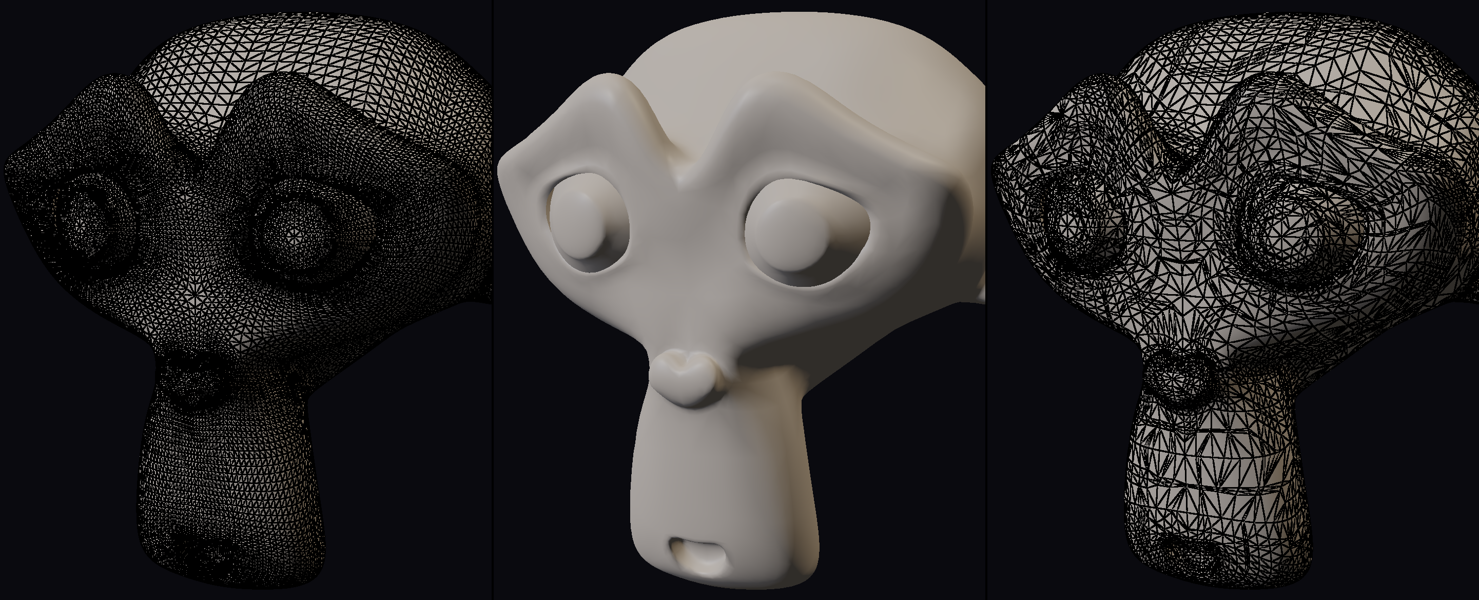
The header image shows Catmull-Clark in action. The left image is the uniform tessellation wireframe, the right is the adaptive tessellation wireframe, and the middle is the adaptive version shaded.
In this post, we’re going to discuss a new approach to this problem, as a spiritual descendant of the feature-adaptive subdivision work from Brainerd et al. [2]. The key innovation of their approach is to split the problem into two parts:
- Tessellation: Dicing a mesh using hardware tessellation.
- Subdivision: Given a barycentric coordinate on a face, calculating that limit position and normal.
We’ll be taking it one step further, using compute tessellation (from the previous post) as well as a novel way of calculating the limit position of the surface. But before we get into that, we need to go over the background of Catmull-Clark, as well as the innovations over the last few decades.
Here you can open the live WebGPU Catmull-Clark viewer. Or if you prefer you can download the viewer as a standalone zip. The code is MIT licensed.
Catmull-Clark Background
The original algorithm is quite simple and elegant. At each level, we start with a polygon mesh. Each iteration requires three steps:
- For each face, create a new point F at the centroid of each face.
- For each edge, create a new point E based on the previous level and the new F points.
- For each vertex, create a new point V based on the new E/F points and the previous level vertices.

Semisharp Creases and Vertices
One of the difficulties with vanilla Catmull-Clark is generating sharp edges like bevels. You can do it by adding extra edge loops where you need them, but that adds complexity and authoring cost. As such, semisharp rules have been proposed and gained wide adoption [3].
Edges and vertices have both a smooth rule (original Catmull-Clark) and a sharp rule, where each vertex and edge has a semisharp weight. If the weight is, say, 3.6, then the first 3 subdivisions would use the sharp rule. The fourth would use a 60%/40% split between the sharp and smooth rules, and the rest would be smooth only.
The image below shows the comparison between the sharp and smooth rules for both vertices and edges.

Here is a screenshot of semisharp edges and creases from the actual demo.
Bicubic B-Splines
Catmull-Clark subdivision has a very interesting property. If a set of vertices makes a clean 4x4 grid of vertices, then the inner quad is called “regular”. And a regular quad can actually be evaluated analytically with a simple formula: the Bicubic B-Spline. Given any (u, v) value inside that quad, we can evaluate it as a simple polynomial.

We can apply any tessellation we desire to that quad, and analytically evaluate the position and normal. The hard part is calculating the limit positions and normals of irregular polys.
Semisharp Edges with Bicubic B-Splines
Can we use the Bicubic B-Spline evaluation for quads that have a semisharp edge or vertex? It depends.
If we have a single semisharp edge, then we can use an analytic evaluation. In Nießner, Loop, and Greiner [7] they show that a single cubic B-Spline can be made equivalent to the semisharp rules by applying a change of basis. Since a Bicubic B-Spline is separable, we can simply rotate the patch so that the one semisharp edge is along the same axis. So, if a regular quad has one semisharp edge, we can still evaluate it analytically. But if the quad has multiple semisharp edges or a single semisharp corner, then we have to treat the quad as irregular.

Feature-Adaptive Subdivision
The key innovation comes from Feature-Adaptive Subdivision by Nießner, Loop, Meyer, and DeRose [1]. In the scene below, we have an irregular vertex in pink that touches 5 quads. Look at what happens as we subdivide it.

As it subdivides, only quads that touch the irregular vertex stay irregular. The other new quads are regular by construction. If we wanted to apply pure subdivision, we would need 4x as many vertices at each level. But if we only subdivide at the irregular vertices, each level requires the same number of points.
The original feature-adaptive paper [1] used special rules to cut the mesh. But the Brainerd et al. [2] approach used a very clever idea. For each quad, they could store the feature-adaptive patches as a quadtree.
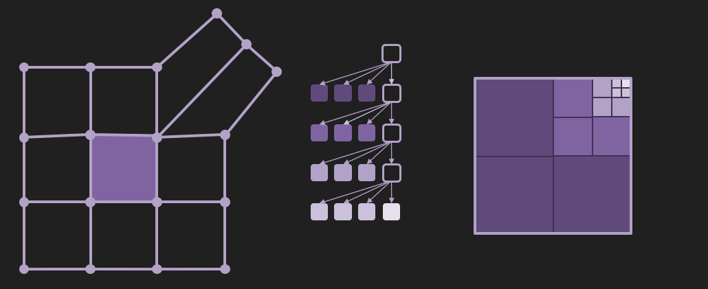
They use standard hardware tessellation to handle the topology. And then each vertex is evaluated in the domain shader by traversing the quadtree and evaluating a point on the proper regular patch.
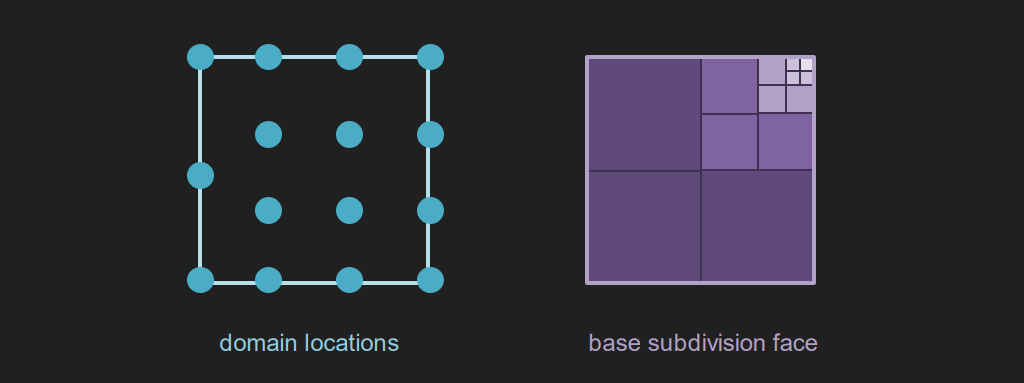
For any given (u, v) coordinate on the quad, they can traverse a tiny quadtree and find the regular patch that belongs to that point. There is one exception: they only calculate a certain number of subdivision levels. At the finest subdivision level, in the quad touching the vertex, the patch cannot actually be evaluated. However, in practice those points are never sampled.

As a final detail, how are those control points calculated each frame if the mesh deforms? It would be quite messy to actually run Catmull-Clark subdivision on those irregular points each frame. However, Catmull-Clark has one other interesting property: any given control point on a face (at any subdivision level) is a linear combination of control points in the one-ring around it. So the algorithm doesn’t need to actually run the Catmull-Clark iteration each frame. Instead, the weights can be precalculated. Then upon deformation, each bicubic patch control point is evaluated as a linear combination of nearby vertices, analogous to joint skinning.
This is exactly what Pixar’s OpenSubdiv library [4] does. The Stencil Tables hold the precomputed limit-stencil weights, while the Patch Tables hold the feature-adaptive patches. Per-frame deformation reduces to applying the stencils to the moving control points.
Tradeoffs
There are a few implicit tradeoffs with this approach.
- The original algorithm uses quads. This means that for hybrid triangle meshes, we need to do one subdivision up front to convert the hybrid quad/triangle mesh into quads only.
- For dynamic tessellation, fractional-even is used, which requires a minimum tess factor of two. Combined with the previous point (one subdivision applied as a pre-process), we need to have a 4*4=16x expansion of points at a minimum.
- Even though the number of irregular points increases linearly at each level, it's still quite a lot. For an irregular vertex, each adjacent quad requires 24 points per level (12 unique ones if shared). For 8 levels, a valence-5 irregular point would require 5*12*8=480 control points per irregular vertex. This isn't a dealbreaker, but it adds up fast.
- Hardware tessellation: I'll leave this discussion as an exercise for the reader.
Irregular subdivision
Instead, we’re going to use a different algorithm for creating patches around the irregular points. Suppose we have a single irregular point, in this case adjacent to 5 quads. Here is the original geometry.

Then assume that we have already subdivided it once. From there, we can apply the Catmull-Clark steps as normal: face points, then edge points, then vertex points.

However, take a close look at these new points. For each of the original quads at this subdivision level, we have three regular quads (in pink) and one irregular one (in white). But more importantly, we can discard the outer row, and our points are ready for the next iteration.

Left: After a full irregular iteration, each original quad has three regular patches in pink, and one irregular patch in white. Right: The outer points can be discarded so that we can iterate on the next level.
Whereas the Brainerd et al. feature-adaptive approach [2] stores a table of points, we can instead store only the ring at the first level (6 points per poly, single level) and recalculate the finer levels on the fly. Conveniently, if we use one thread per valence, we can pack multiple irregular vertices into one 64-thread workgroup.
The full algorithm follows the pattern below. We start with the original mesh at import time (Level 0), then we store the lookup tables for Level 1. Our first iteration generates the points at Level 2. From there, we can continue iterating until we reach the desired subdivision level.

All irregular vertices have the same pattern, so we do not need a special quadtree. Instead, we can determine which level we are in by using -log2(max(u, v)).

We have one last detail: we don’t actually have a valid Bicubic B-Spline in the white area. To solve this, we make sure to calculate the limit point of all irregular vertices using a table. To calculate P, we first calculate B on the patch. P is then found by interpolating C and B.

There are potentially other approaches. In the past I looked at variations such as filling the missing area with a G1 patch. In theory it sounded like a good idea, but in practice it created star-shaped specular highlights. I’ve found that a straight linear interpolation with the limit point looks cleanest visually.
Regions
Instead of using a quadtree, we have an explicit two-step process. First, each quad is split into several regions, and each region is either regular or has an indirection to a section of an irregular ring. In the case below, the middle quad has 4 regions. Three are orange and form regular patches. The other pink one has an indirection to the irregular ring.

Triangles
What do we do with triangles? We actually need to subdivide them twice. Subdividing them once results in a mesh that is all quads, but the newly created point in the middle is irregular. So the irregular points need to be subdivided one more time. Note that the three vertex points from the original triangle may or may not be irregular. However, the quads attached to them will need to be subdivided twice regardless.

Primitives
Altogether, we have four ways of splitting a primitive into regions. Quads can be classified as Regular, Subdiv 1, or Subdiv 2, with 1, 4, and 16 regions, respectively. Triangles are subdivided twice, into 12 regions total.

Adaptive vs. Fixed tessellation on Suzanne
Below are two side-by-side comparisons of Suzanne (507 source verts, 968 source tris). In each pair the solid shading is visually indistinguishable, even though the adaptive pass outputs roughly half as many triangles.
The first comparison is the full head in frame. The wireframe shows the adaptive pass concentrating triangles around the areas of high curvature.
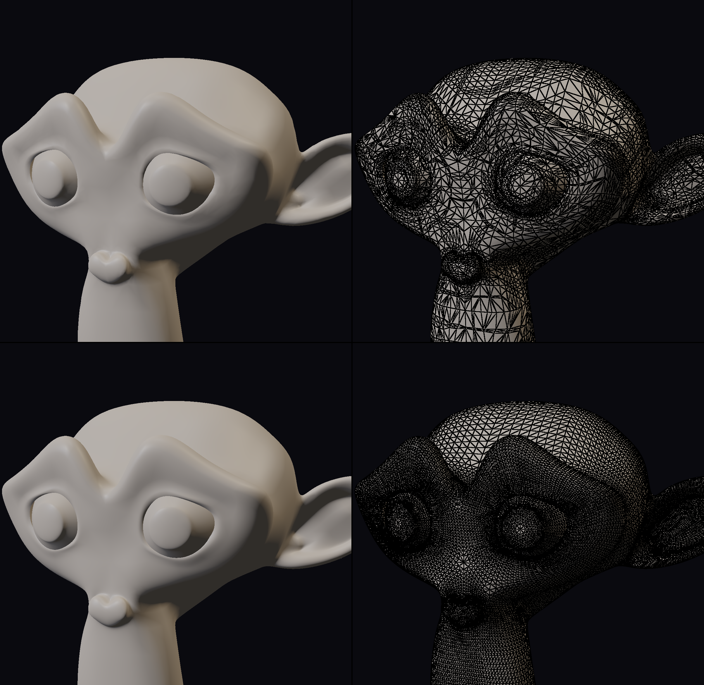
Suzanne, full-head view. Top: Adaptive Curvature. Bottom: Fixed.
| Fixed | Adaptive Curvature | |
|---|---|---|
| Output verts | 43,560 | 24,622 |
| Output tris | 61,952 | 30,526 |
The second comparison pushes the camera in close on the top of the head, so most of the mesh ends up behind the camera or off-screen. Adaptive pulls density off the unseen regions and spends it on the visible silhouette, resulting in more density at the silhouette than the uniform fixed pass despite using about half as many triangles overall.
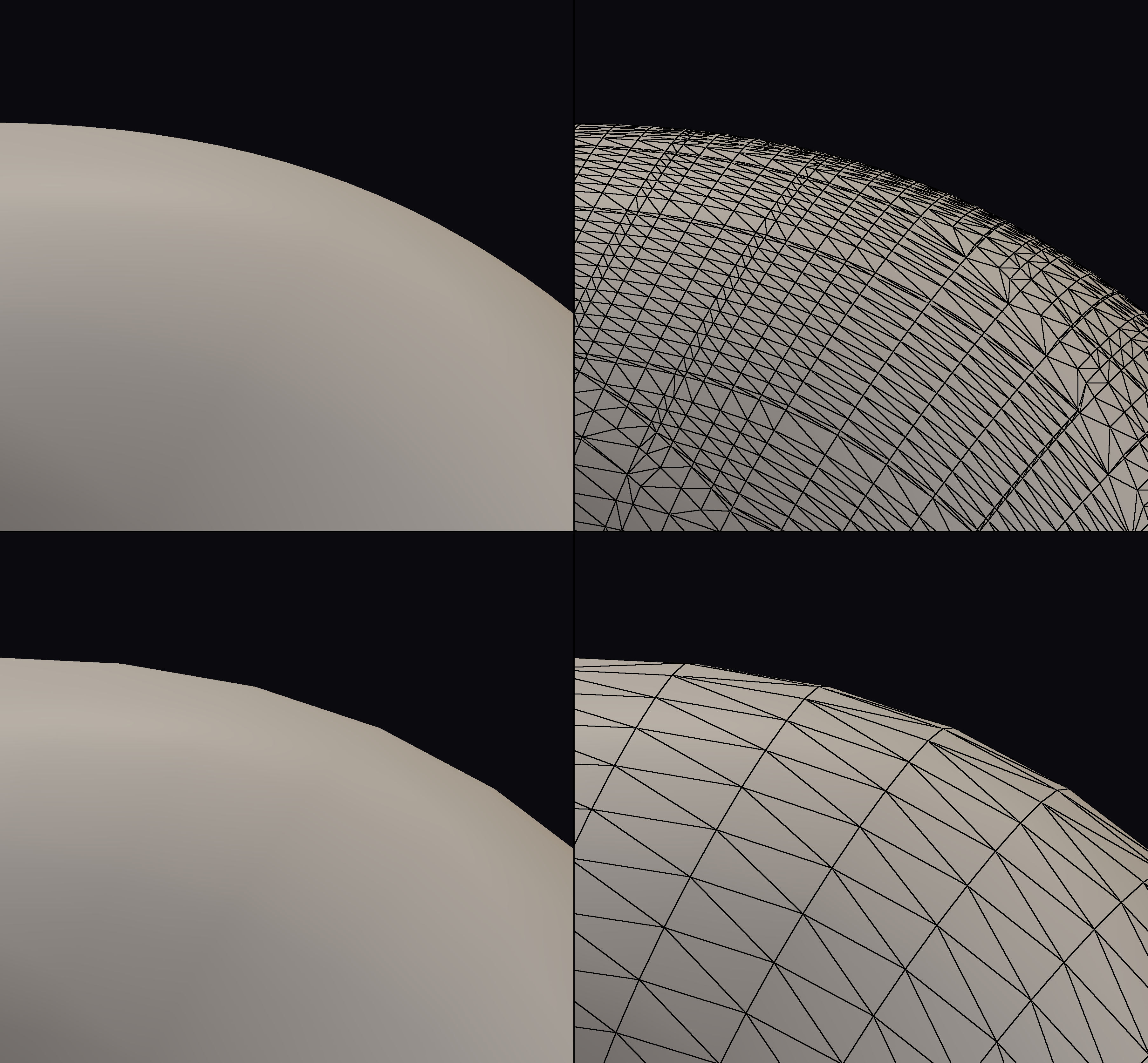
Suzanne, silhouette zoom on the top of the head. Top: Adaptive Curvature. Bottom: Fixed.
| Fixed | Adaptive Curvature | |
|---|---|---|
| Output verts | 43,560 | 19,818 |
| Output tris | 61,952 | 29,918 |
Performance
Here is the compute cost for four different test models. These were measured on my desktop machine, which has an NVIDIA RTX 3070. The passes include the compute cost, but not the full rendering time. The subdivision pass calculates the control points, but does not perform the actual point evaluation. If the model were not deforming, we could calculate the subdivision pass once and reuse those points every frame.
| Mesh | Output tris | Subdivision | Tessellation | Sub + Tess |
|---|---|---|---|---|
| suzanne | 15.9M | 0.037 ms | 3.368 ms | 3.405 ms |
| bigguy | 11.9M | 0.025 ms | 2.171 ms | 2.196 ms |
| monsterfrog | 10.6M | 0.028 ms | 2.014 ms | 2.042 ms |
| imrod | 14.2M | 0.139 ms | 3.243 ms | 3.382 ms |
Note that the subdivision cost of imrod is much higher than the other models because it is roughly evenly mixed between triangles and quads, and each triangle requires two subdivision levels of control points. If we were to author meshes specifically for subdivision using this algorithm, my advice would be to only use quads and never use triangles.
Here are some numbers from the Edge-Friend paper [5], which has an implementation of both Edge-Friend and DV21 [6]. Their numbers are on a 4080, whereas my tests are on a 3070. The last row includes a 2.4x scale as a very coarse estimate of this algorithm’s performance on a 4080.
Big Guy.
| Implementation | Hardware | tri / ms |
|---|---|---|
| Edge-Friend | RTX 4080 | 11,101,308 |
| DV21 | RTX 4080 | 2,984,523 |
| Adaptive Compute | RTX 3070 | 5,424,954 |
| Adaptive Compute (2.4x) | — | ~13,019,890 |
Imrod.
| Implementation | Hardware | tri / ms |
|---|---|---|
| Edge-Friend | RTX 4080 | 10,820,778 |
| DV21 | RTX 4080 | 2,915,844 |
| Adaptive Compute | RTX 3070 | 4,207,597 |
| Adaptive Compute (2.4x) | — | ~10,098,233 |
In order to properly compare with Edge-Friend, we would have to run the same algorithm on the same computer. The 2.4x scalar is an estimate, but could be more or less depending on whether the bottleneck is bandwidth or ALU.
Acknowledgements
I have to give a big thanks to Natalya Tatarchuk and Gregory Mitrano, who were both invaluable in discussing and working through the various problems and corner cases of this approach.
References
- Nießner, Loop, Meyer, and DeRose, "Feature-Adaptive GPU Rendering of Catmull-Clark Subdivision Surfaces", ACM Transactions on Graphics 31(1), 2012.
- Brainerd, Foley, Kraemer, Moreton, and Nießner, "Efficient GPU Rendering of Subdivision Surfaces using Adaptive Quadtrees", ACM Transactions on Graphics 35(4), 2016. See also the GDC 2017 talk slides.
- DeRose, Kass, and Truong, "Subdivision Surfaces in Character Animation", SIGGRAPH 1998.
- Pixar, OpenSubdiv, https://opensubdiv.com/docs/intro.html.
- Kuth, Bürger, Wand, and Stamminger, "Edge-Friend: Fast and Deterministic Catmull–Clark Subdivision Surfaces", Computer Graphics Forum 42(8), 2023.
- Dupuy and Vanhoey, "A Halfedge Refinement Rule for Parallel Catmull–Clark Subdivision", High Performance Graphics 2021. Code: github.com/jdupuy/HalfedgeCatmullClark.
- Nießner, Loop, and Greiner, "Efficient Evaluation of Semi-Smooth Creases in Catmull-Clark Subdivision Surfaces", Eurographics 2012, pp. 41–44.