Introduction
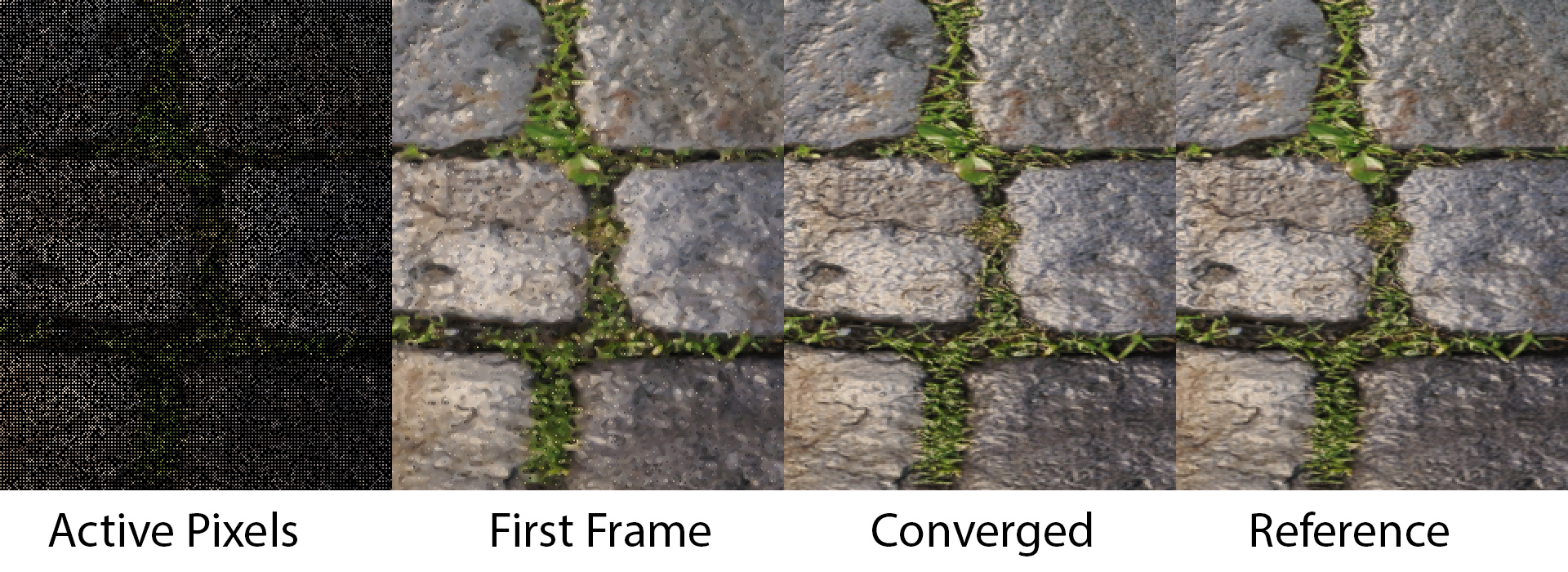
There are some very interesting tradeoffs involved in visibility rendering, and many techniques to explore. The first post was an overview of visibility rendering and how it could be optimized with material graphs. The second is a new technique for decoupling geometry sampling rate from shader sampling rate for better anti-aliasing. This third one discusses another way of separating the geometry sampling rate from the shading sampling rate: Variable Rate Shading.
Adventures in Visibility Rendering
- Part 1: Visibility Buffer Rendering with Material Graphs
- Part 2: Decoupled Visibility Multisampling
- Part 3: Software VRS with Visibility Buffer Rendering
- Part 4: Visibility TAA and Upsampling with Subsample History
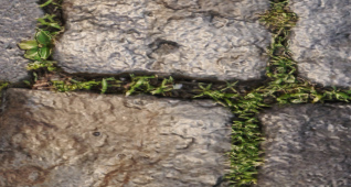
Hardware Variable Rate Shading (or VRS for short) allows GPUs to perform shading and geometry sampling at different rates. It is a relatively new feature, but is now supported on AMD [1], Intel [4], and NVIDIA [7] GPUs. Here is a single zoomed-in example frame with Forward Rendering and TAA:
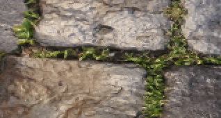
Next, here is the same shot with 2x2 Hardware VRS enabled. It uses different sampling points than the 1x image, with each 2x2 shading point being the average of the four original sample points.
However, with Visibility rendering, we can take a different approach. Instead of changing the samples like hardware VRS does, we can choose a subset of the sample points that we would normally render.
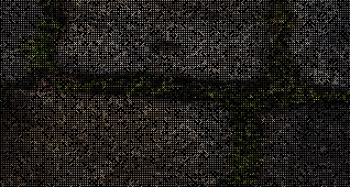
We can then perform a custom interpolation of those points which gives a blurry result.

We can then randomize the sample points each frame. Since the samples are in the same positions as the 1x frame, it will converge to the original reference frame over time if nothing is moving. This feature is in contrast to Hardware VRS which would converge to a blurrier image than the original. Here is the final converged frame:

In addition to higher converged quality than Hardware VRS, this approach has performance benefits as well, especially as the triangle density increases.
Prior Art
In particular, there are several options to vary the shading rate over the image with hardware VRS [8]. Additionally, since you can specify a screen-space mask for VRS level, you can adaptively apply conservative or aggressive sampling rates based on content, as was done in the latest Gears 5 [9]. There are also software versions, such as Call of Duty: Modern Warfare which emulated 2x2 pixel quads using 4xMSAA [2]. Additionally, Marissa du Bois from Intel [3] has a good overview video discussing the technique, practical considerations, and the integration with UE4. In the second half of that video, John Gibson from Tripwire discusses performance numbers from their game, Chivalry 2. Tomasz Stachowiak also implemented an impressive system via GCN hacking to group shaders by occupancy, with a VRS algorithm when data is shared along the same pixel quad [10].
It’s a very nice win. The API is very easy to enable, and in many cases you can get better performance without any other work. If it looks the same, but is faster, then of course you should do it. But there are ways we can improve the technique by doing it ourselves, in software.
As mentioned previously, we can use the same sample positions as the 1x reference image, so that our image converges to the non-VRS result. Also, Visibility VRS is able to solve some of the performance inefficiencies with Hardware VRS. What inefficiencies does Hardware VRS have? Well, if you thought we were done talking about quad utilization then I have some bad news for you.
Quad Utilization
In the previous post, there is a discussion about how rendering is broken up into quads. With regular 1x rendering, the rasterizer will split this triangle into 2x2 quads, and the grey pixels will be helper lanes that need to run.
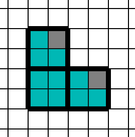
We end up with 3, 2x2 quads. One for the upper-left, bottom-left, and bottom-right. The grey pixels do not contribute to the final image, and exist only to provide partial derivatives to the UVs of pixels that will actually appear on the screen.

So, what happens if we render this same triangle with 2x2 VRS? The rasterizer will think of each 4x4 block of pixels as a single 2x2 quad, like below.
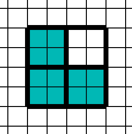
Then it will spawn a single pixel shader quad, where the upper-right is a helper lane.

After the pixel shader is run, it will apply each of those colors to each 2x2 block in the original image. Suppose we have a large triangle in purple, like below. In the regular non-VRS case, if the triangle touches a single pixel in a 2x2 square, then the other points need to be rendered as helper lanes. These lanes are shown in grey.
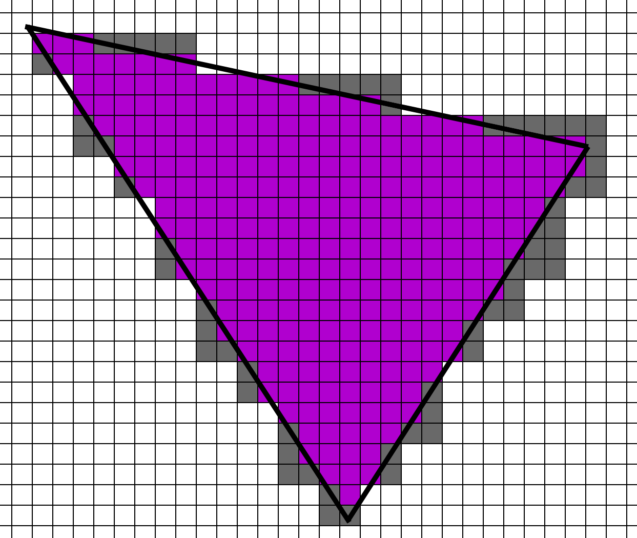
This process “rounds up” when VRS is enabled. With 2x2 VRS, if this triangle touches a single pixel in a 4x4 grid, the rest must be filled in with helper lanes. Said another way, if a triangle touches at least one pixel of a 4x4 block, then the 4x4 block must be rendered.
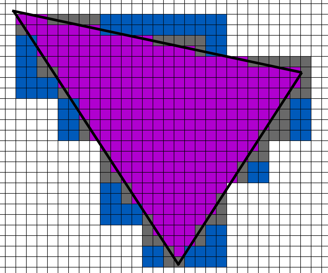
When rendering this triangle with 2x2 VRS, the rasterizer needs to find all the 4x4 blocks that are touched by this triangle. Then those 4x4 blocks becomes quads which get sent to the pixel shader. The 2x2 groups of blue pixels become a helper lane in the VRS pixel shader quad. Although that 4x4 block of pixels will only spawn a single 2x2 quad to process.
So, how many times does a pixel shader need to run for a large triangle? As discussed previously, in the standard non-VRS case, a Forward renderer would call the pixel shader once per pixel. It would be the same for the Material and Lighting pass of a Deferred renderer, as well as a Visibility renderer. However, what about the 2x2 VRS case?
In a Forward renderer, we would expect each pixel shader to run once per 2x2 quad, which would mean 0.25 pixel shader invocations per pixel. For Deferred, the Material pass would be rasterized at 0.25 pixel shader invocations per pixel, but the Lighting pass would run at 1x since it isn’t rasterized. Yes, there are ways to run Lighting at lower rate as was performed in Gears 5 [9], but we’ll skip those details for now.
What about visibility though? Can we render at 0.25 invocations per pixel? Sure, why not? We can choose a subset of pixels, light those, and interpolate the in-between pixels.
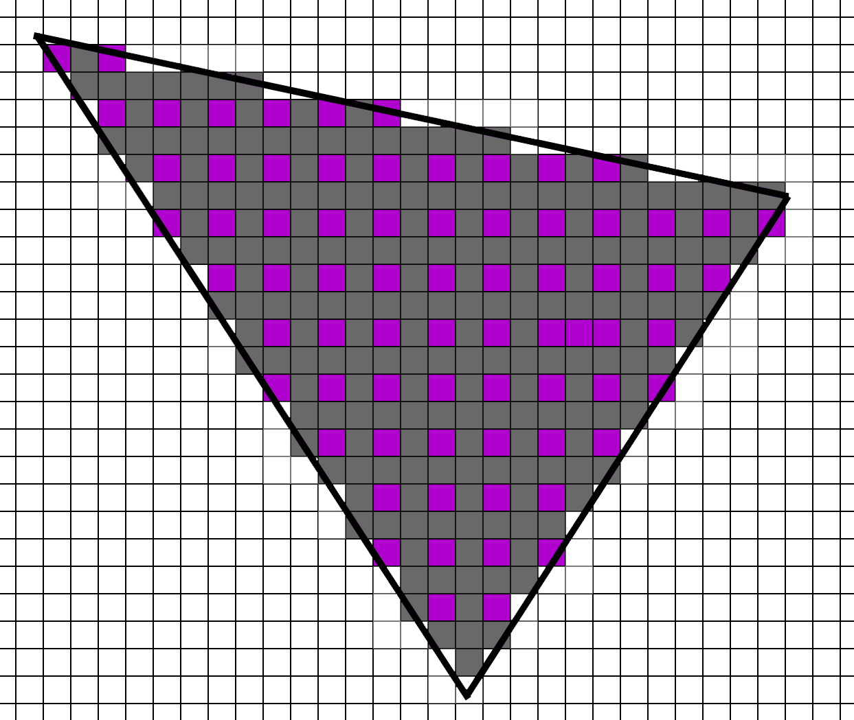
We will have extra work to do, but we can absolutely do it. Also, note that we do not need helper lanes since we are able to calculate uv derivatives analytically.
Here is the table showing how many times the Lighting and Material evaluation would run for Forward/Deferred/Visibility in the non-VRS and 2x2 VRS versions.
Approximate shader function invocations per pixel for large triangles:
| Material (non-VRS) | Lighting (non-VRS) | Material (2x2 VRS) | Lighting (2x2 VRS) | |
|---|---|---|---|---|
| Forward | 1x | 0.25x | ||
| Deferred | 1x | 1x | 0.25x | 1x |
| Visibility | 1x | 1x | 0.25x | 0.25x |
Simple enough. Forward and Deferred Material can run at 0.25x rate thanks to Hardware VRS. Visibility can run at 0.25x rate with our own Software VRS solution. And Deferred Lighting runs at 1x since it is in a full-screen pass, although it could be optimized as it was done in Gears 5.
Let’s move on to small triangles. In the non-VRS case, any 1-pixel triangle becomes a 2x2 quad with 1 active lane and 3 helper lanes.
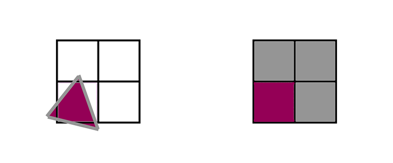
What happens to that same tiny triangle in the 2x2 VRS case? Unsurprisingly, the exact same thing happens. The pixel shader converts it to a 2x2 quad with 1 active lane and 3 helper lanes, just like the non-VRS case.
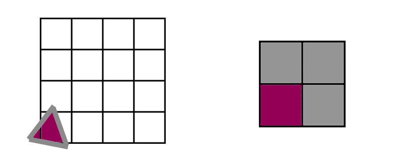
For tiny, 1 pixel triangles, the VRS and non-VRS cases are the same. A tiny triangle will always need 1 active lane, which will require a quad with 3 helper lanes. But what about for Visibility rendering?
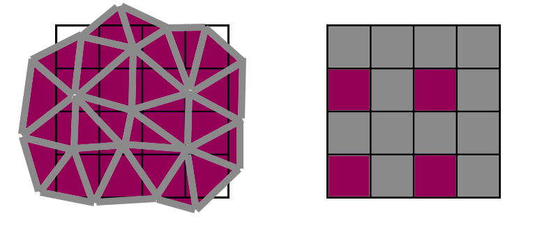
With visibility, we can still render at 0.25 shader invocations per pixel. Since the choice of pixels to run is arbitrary, we can use the same algorithm as the large triangle case. We only need to render a subset of the pixels and we can interpolate the rest. The size of the triangle is irrelevant. Here is the table of shader invocations per pixel.
Approximate shader function invocations per pixel for 1-pixel triangles:
| Material (non-VRS) | Lighting (non-VRS) | Material (2x2 VRS) | Lighting (2x2 VRS) | |
|---|---|---|---|---|
| Forward | 4x | 4x | ||
| Deferred | 4x | 1x | 4x | 1x |
| Visibility | 1x | 1x | 0.25x | 0.25x |
And that is really the key idea of Visibility rendering with VRS. With tiny triangles, the Forward and Deferred Material pass have to render 4 pixel shader invocations per pixel due to quad utilization, regardless of VRS. But with visibility rendering we can maintain 0.25 shader invocations per pixel in both cases.
Finally, what about more typical, 10 pixel triangles? Let’s start with this one again:
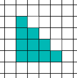
In that case, the triangle fits perfectly into a 4x4 block of pixels, and will create exactly one quad. However, there are 16 ways for that triangle to align with the 4x4 grid.

There is exactly 1 way for the triangle to fit perfectly inside a single 4x4 block, but 6 ways to touch 2 blocks, 6 ways to touch 3 blocks, and 3 ways to touch 4 blocks. That means this shape of triangle will spawn 10.75 pixel shader lanes on average (active + helper).
| Touched 4x4 Blocks | Variations |
|---|---|
| 1 | 1 |
| 2 | 6 |
| 3 | 6 |
| 4 | 3 |
Let’s take a look at a longer, thinner shape.
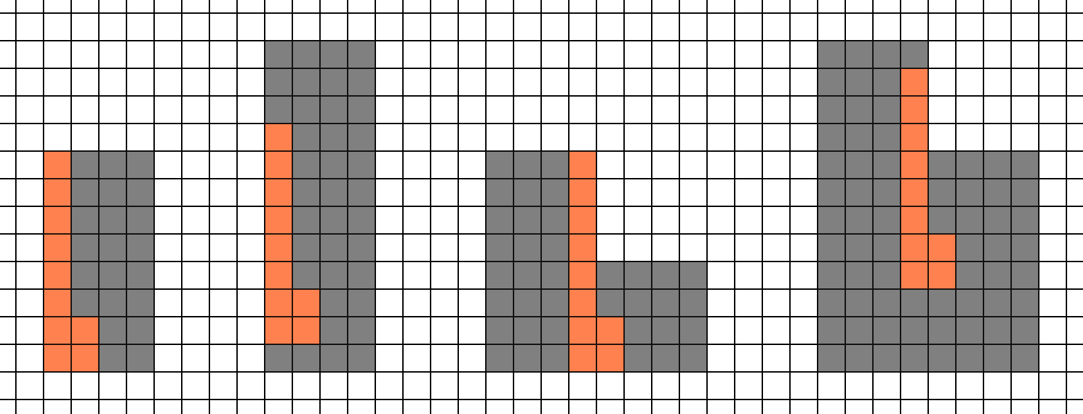
This one is a little worse. There is no way for it to hit exactly one 4x4 block, and on average this shape will spawn 12.25 pixel shaders.
| Touched 4x4 Blocks | Variations |
|---|---|
| 1 | 0 |
| 2 | 3 |
| 3 | 10 |
| 4 | 2 |
| 5 | 1 |
For our two shapes, they will on average require 10.75 and 12.25 pixel shader invocations each. Don’t forget: The original triangle is only 10 pixels. So even though we are trying to render the shading rate at 1/4 of the geometry rate, we still actually have more shader invocations than we have pixels.
If you remember from the previous post, with non-VRS we have about 2x shader invocations per pixel. For simplicity, let’s say that our 10-pixel triangles at 2x2 VRS require 1x shader invocation per pixel. And for Visibility rendering, we can easily get 0.25x shader invocations per pixel.
Approximate shader function invocations per pixel for 10-pixel triangles:
| Material (non-VRS) | Lighting (non-VRS) | Material (2x2 VRS) | Lighting (2x2 VRS) | |
|---|---|---|---|---|
| Forward | 2x | 1x | ||
| Deferred | 2x | 1x | 1x | 1x |
| Visibility | 1x | 1x | 0.25x | 0.25x |
Based on this analysis, we would expect performance for Forward, Deferred, and Visibility to be similar for very large triangles. However, as triangles get closer to 10 we would expect Visibility to be faster. And then as triangles shrink all the way to a single pixel, Visibility should be the winner due to quad utilization. Of course, before we do that, we should probably discuss how to actually do VRS in software with Visibility buffers.
Software VRS with Visibility
At a high level, we are going to mark pixels as either on or off. Pixels marked as on will be accumulated into the Visibility Material pass which will generate a sparse GBuffer. The sparse GBuffer will be lit by the Lighting pass. And then we will unpack the sparse lighting and fill in the holes. Then we can pass that image to TAA which can magically fix everything. Joking, not joking.
As an example, the selected pixels will look like this:

The single reconstructed frame will look like this:

And the final frame after TAA will look like this:

The first question is: How should we reconstruct the image from sparse points? I tried several options, and many variations of bilateral upsampling, but the approach which worked the best was from the Deferred Active Compute Shading papers, from Ian Mallet, Cem Yuksel, and Larry Seiler [5,6]. Their key idea was to first render a full GBuffer, but perform lighting at variable rate using iterative passes. Their algorithm starts by calculating lighting at every 4th sample in X and Y, like so:
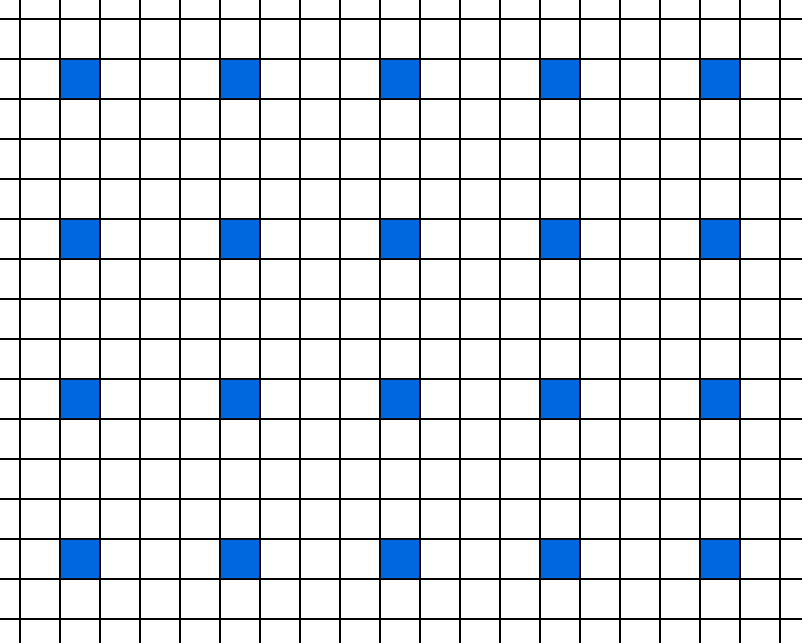
The next step is to fill in the missing pixels. For a pixel like the one below, we can interpolate the value from the 4 neighbors.
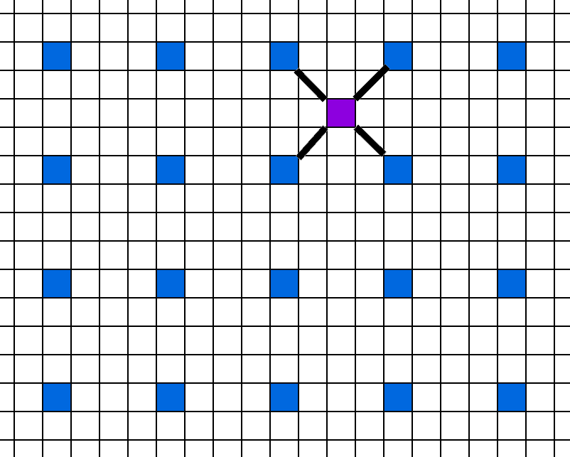
They had one very, very interesting innovation. Since the data is there, they could choose to either calculate or interpolate the pixel on-the-fly. They would compare the values of all 4 neighbors, and if they are close enough, interpolate. But if the GBuffer data was different, they would perform the more expensive full lighting calculation. It’s a very cool approach, and I’d recommend reading both papers. For each value in between, they choose new colors either by interpolating or calculating it directly.
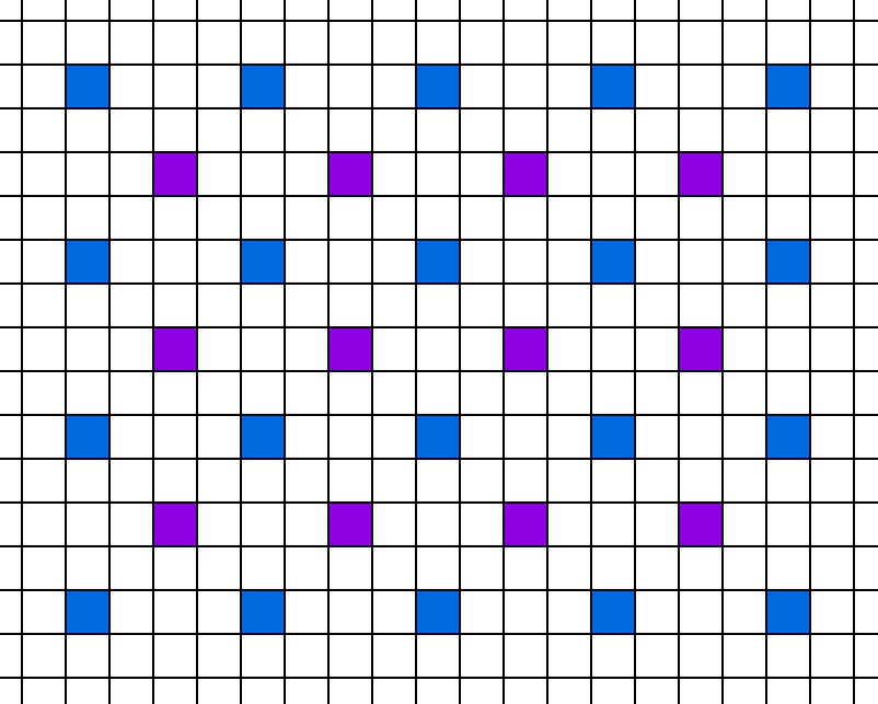
This continues for a 2nd step…
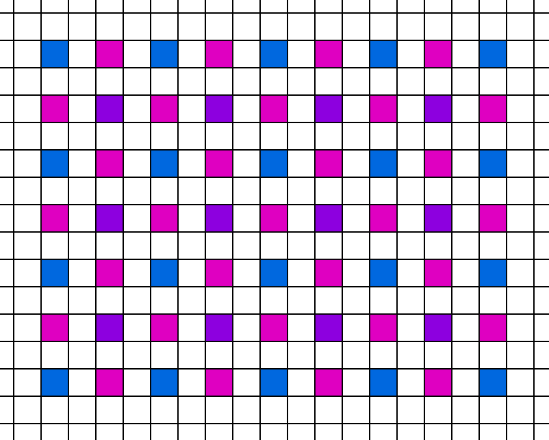
…and a 3rd step…
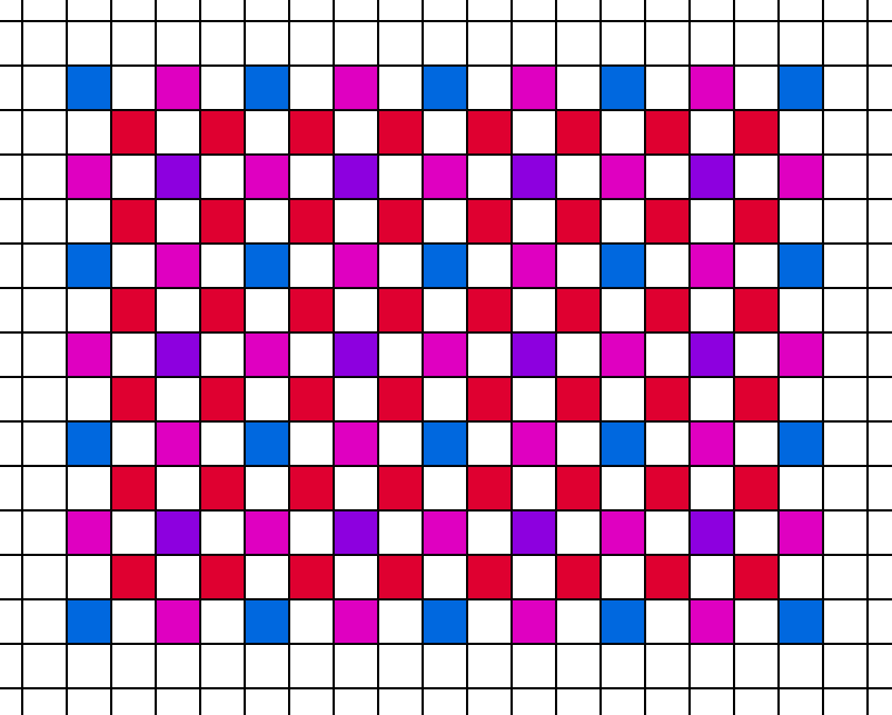
…and a 4th step…
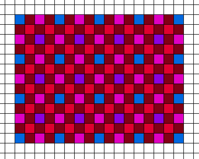
…until the image is complete. Waiting to decide between interpolating and lighting a pixel until the neighbors were lit is not practical in this Visibility buffer implementation. So for our variation, we will start with an image after the sparse lighting pass.
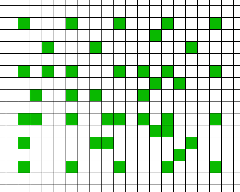
The green pixels are the locations where we calculated a lighting value. Then for each pass, we fill in the blanks. What algorithm should we use for this new pixel?
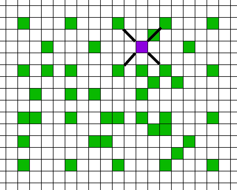
The common approach would be to use the smaller absolute difference, as has been used in image debayering. It’s probably easiest to explain with code:
float3 InterpolatePrimaryCrossColorMerged(
	uint matC, uint mat0, uint mat1, uint mat2, uint mat3,
	bool validC,
	float3 colorC, float3 color0, float3 color1, float3 color2, float3 color3)
{
  float4 color = 0.0f;

  float4 temp0 = (matC == mat0) ? float4(color0, 1) : float4(0, 0, 0, 0);
  float4 temp1 = (matC == mat1) ? float4(color1, 1) : float4(0, 0, 0, 0);
  float4 temp2 = (matC == mat2) ? float4(color2, 1) : float4(0, 0, 0, 0);
  float4 temp3 = (matC == mat3) ? float4(color3, 1) : float4(0, 0, 0, 0);

  float4 avg0 = .5f*(temp0 + temp1);
  float4 avg1 = .5f*(temp2 + temp3);

  bool bothGood0 = temp0.w >= .75f;
  bool bothGood1 = temp1.w >= .75f;

  if (bothGood0 && bothGood1)
  {
    float diff0 = abs(dot(float3(1, 2, 1), temp0 - temp1));
    float diff1 = abs(dot(float3(1, 2, 1), temp2 - temp3));
    color = diff0 < diff1 ? avg0 : avg1;
  }
  else if (bothGood0 && !bothGood1)
    color = avg0;
  else if (!bothGood0 && bothGood1)
    color = avg1;
  else
    color = avg0 + avg1;

  if (color.w < .25f)
    color = float4(color0 + color1 + color2 + color3, 4);

  color.xyz *= rcp(color.w);

  if (validC)
    color.xyz = colorC;

  return color.rgb;
}
Note that we are passing in both the draw call IDs of the center pixel and the 4 neighbors, and we are only going to interpolate using neighbors that are from the same draw call ID. There are two sets of pairs that we can use to interpolate this pixel. A pair is considered “good” if both pixels are on the same draw call ID as the pixel we want to calculate. If both pairs are good, then we interpolate using the “better” pair, where the “better” pair is the one with a smaller absolute difference. If only one pair is good, then we use that pair. And if neither pair is good then we just add up the pixels and hope for the best.
In retrospect, selecting pairs for interpolation using smaller absolute differences likely wasn’t the best choice. In the raw images there are a number of single pixels that look a bit like noise. Those are pixels that were significantly brighter or darker than the average. Thus when interpolating the nearby pixels, those pixels were not used since the other pair was always chosen. So I might switch to a straight average of pixels, or a hybrid approach. It needs more investigation.
The advantage of this approach is that interpolation is fast, as it only requires the nearby 4 pixels. But it is also edge-aware so colors will not bleed. What happens if all 4 neighbors are on a different draw call ID? In the worst case, we can take the average and accept the bleeding. But we can actually stop it from happening in the first place. When selecting which pixels to calculate/interpolate earlier in the frame, we can prioritize pixels that do not have any good neighbors, which stops this case from happening.
Using this algorithm, we can proceed with each pass. For each pixel in pass 1, we interpolate the missing pixels.
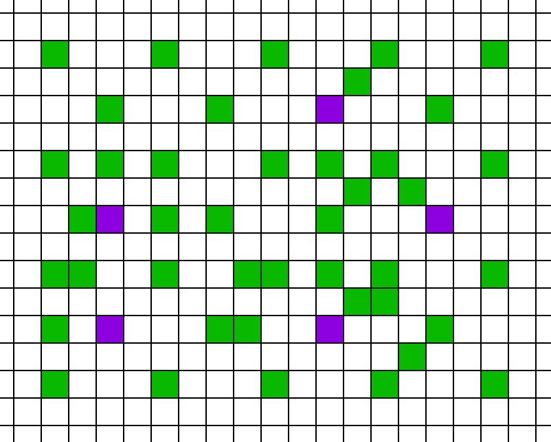
Then we can continue with pass 2…
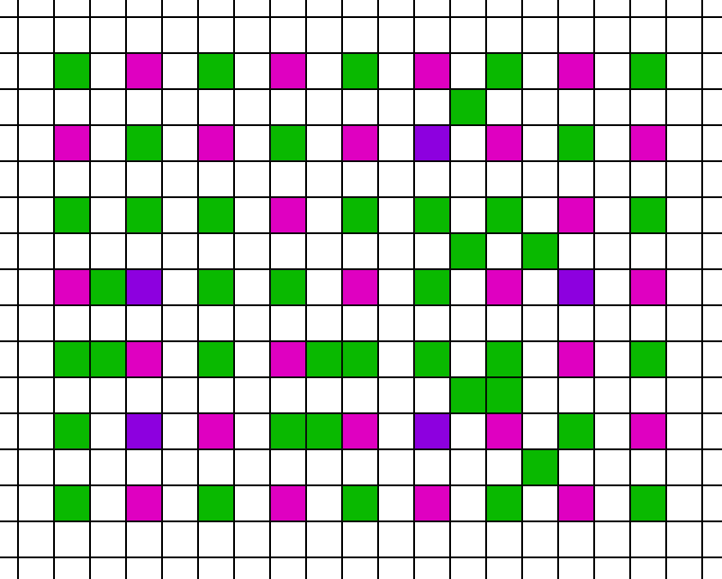
…and pass 3…
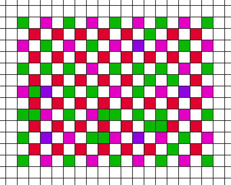
…and pass 4.
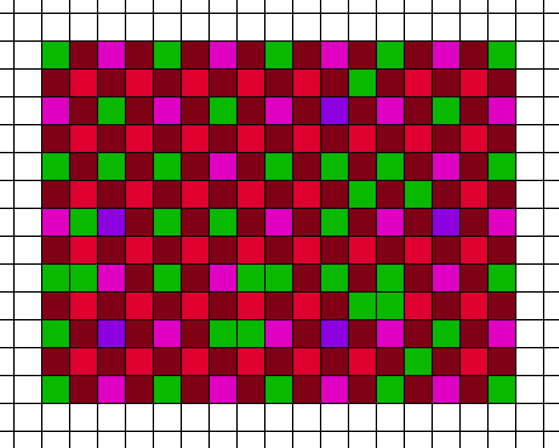
The key advantage of this approach is flexibility. We have complete control of whichever pixels we want to render or interpolate. The only hard rule is that we need to render all the pixels in pass 0 (which is 1/16th of the total pixels). And as a soft rule, we want to render pixels when all 4 neighbors are invalid. Otherwise we can enable/disable pixels by any metric we want.
Convergence
As you might have noticed, we are sampling from different locations than Hardware VRS. In a plain, 1x native render, we would shade all of our sample points in the center of each pixel.
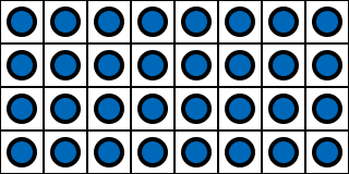
If we enable 2x2 VRS, the sample points move to the center of each 2x2 block. Our final image will be blurrier because we are rendering at lower resolution.
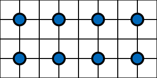
But with this VRS variation, we are rendering at the same sample points as the standard pattern. We are rendering a partial subset at the same locations, as opposed to Hardware VRS which changes the positions.
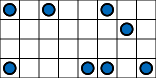
Since we have flexibility, we can choose different sample points in the next frame…
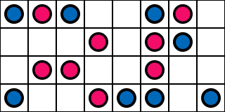
…and the next one…
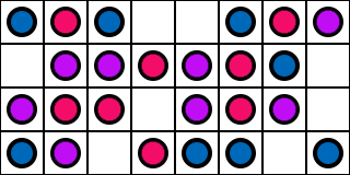
…and the next one.
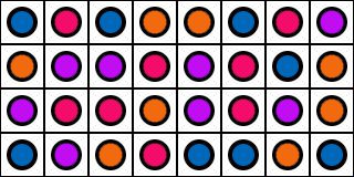
That means if we are careful, we can actually make the image converge to the reference non-VRS image. We can do this by jittering the 4x4 grid every frame, and also giving each pixel a noisy offset to its priority as well.
In the TAA accumulation buffer, we can store a confidence value in the alpha channel. As we get new samples, we increase confidence at that pixel. When we have an interpolated value, if our existing value has low confidence, then we will treat the interpolated value as important. However if we have high confidence, we can disregard interpolated values. As long as we make sure to jitter different pixels in different frames, it will converge properly.
Here is an image from a face scan that I had lying around. The original scan is from Triplegangers which I wrapped to my standard topology with WrapX. This is a closeup of the pores and specular highlight on the model’s cheek. On the left side is the first frame, and the right side is the converged result. The first row is a regular 1x frame, and the second row is Forward with 2x2 VRS. The remaining 4 lines are Visibility with VRS at different ratios.
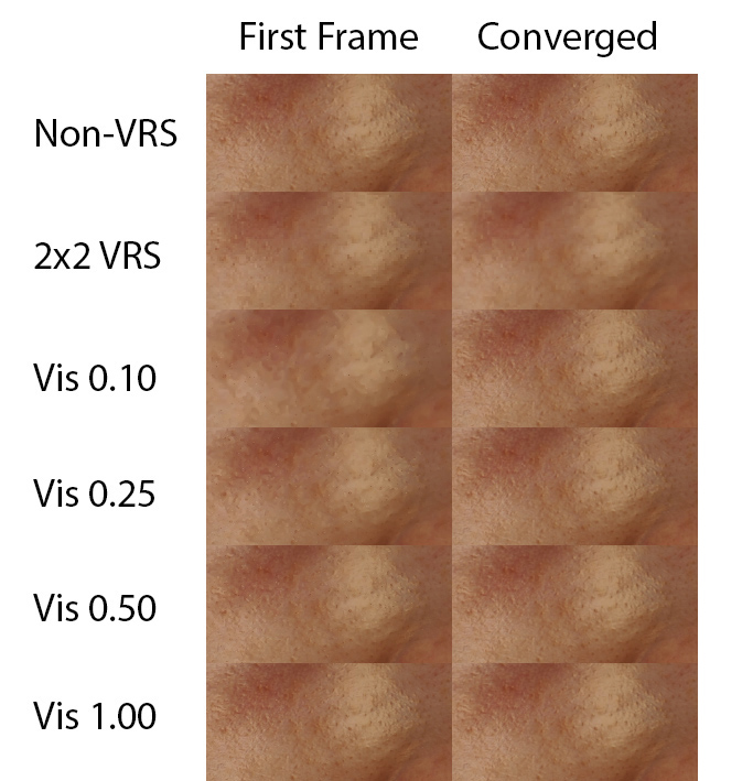
As you can see, the 2x2 VRS version is blurrier both before and after TAA, but the Visibility VRS version converges to the same result as the reference. The rates at 25% and higher converge quite quickly. I wouldn’t recommend actually rendering at 10% rate, as the convergence rate is pretty rough, but it does still get to where it needs to go.
One of the interesting tricks presented in several VRS talks deals with motion. When the object is in motion, it is more difficult for your eye to track it, and that surface will have motion blur applied anyways. So the advice is to have a low sampling rate in areas of high motion, and a high sampling rate in areas of low motion.
However, with Visibility VRS, we can change the tradeoff. We can still have a low sampling rate in high motion. But we can have a low sampling rate in areas of low motion as well, because it will converge in a few frames anyways. We can just have a low shading rate everywhere!
Visiblity VRS fundamentally changes the tradeoff. With standard Hardware VRS, you are trading GPU performance for image quality. Rather, Visibility VRS is trading GPU performance for convergence time, with converged image quality staying constant regardless of shading rate.
The interesting thing for me about Visibility VRS is not that it provides any one particular improvement to render times. Rather, the benefit of Visibility is that all these improvements fit perfectly together. At high triangle counts, Visibility has significant improvements over Deferred/Forward because:
- Visibility at 1x is faster than pure Deferred/Forward due to quad utilization.
- Visibility with VRS gives you a better multipler than rasterized VRS because the rasterizer needs to round up to larger blocks of pixels.
- Visibility with VRS allows more aggressive variable shading rates because it converges to the non-VRS image.
Each of these benefits is great on its own, but the real strength is how they multiply together, which will be discussed in the numbers below.
Choosing Pixels
The last detail to discuss is choosing pixels. In the most recent work, the trend is to analyze the image [7,9], detect how much detail is in that area, and then set the appropriate VRS shading rate. However, we have more flexibility.
We could perform a similar test, determining a cutoff value of quality, but it would cause the performance cost to swing. If you are looking at the sky, you would have GPU cycles idle, whereas when you are looking at a detailed area you would potentially go over your frame time limit.
Instead, we will choose a priority for each pixel, as a 4 bit value. Then we can bin them all up into a histogram and set an explicit threshold value for how many pixels we want shaded in the final image. We can then find the cutoff value, where the cutoff ends up being a float value between 0 and 16. Each pixel tests its priority plus a dither value against the threshold. A value of 3.62 would include all pixels of priority 0, 1, 2, and about 62% of the pixels in priority 3.
Since the interpolation algorithm runs in passes where each pass affects subsequent pixels, pixels in the earlier passes should of course have higher priority. Also, we have pixels that do not share the same draw call with the 4 neighbors, so those need high priority as well. Thus, the base priority looks like this:
| Priority | Pixels |
|---|---|
| 0 | Pass 0 |
| 1 | Zero Neighbors |
| 2 | Pass 1 |
| 3 | Pass 2 |
| 4 | Pass 3 |
| 5 | Pass 4 |
There are several other things we should do. In general, thin objects look quite poor when they do not have enough valid pixels inside them. So we can do a quick search to see if the nearby 4 neighbors are the same draw call in each direction, and then bias the priority so that edges get a priority increase. Here is an example image.
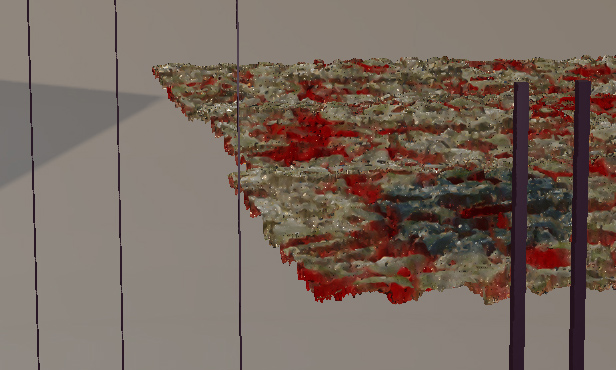
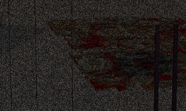
Here are the selected pixels with thin object priority bias off:
And the selected pixels with thin object priority bias on:
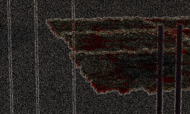
Here is a diff of the image, showing just the pixels that are added by the priority bias.
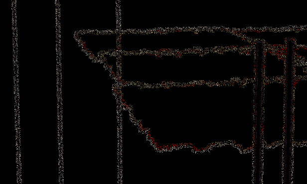
However, since the total number of pixels is constant, adding pixels somewhere means that we have to take away pixels from somewhere else. Here is the reverse of the diff, showing the pixels that were removed by giving priority to edges.
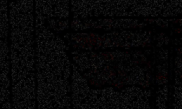
The advantage of this approach is that we can simply choose any combination of metrics we want, and we will always have a consistent number of pixels rendered each frame.
Results
So what do the numbers look like? For the numbers, we will simplify them from previous batches. We will keep track of the length of the PrePass, Material pass, and Lighting pass. But everything else will be in Other. As always, the Material and Lighting passes in Forward are merged together.
| VRS | PrePass | Material | Lighting | Other | Total | |
|---|---|---|---|---|---|---|
| Forward | Off | 0.019 | 1.601 | 0.565 | 2.185 | |
| Forward | 2x2 | 0.019 | 0.442 | 0.564 | 1.025 | |
| Deferred | Off | 0.019 | 1.065 | 0.748 | 0.575 | 2.407 |
| Deferred | 2x2 | 0.019 | 0.402 | 0.733 | 0.579 | 1.733 |
| Visibility | Off | 0.042 | 1.117 | 0.792 | 0.996 | 2.947 |
| Visibility | 25% | 0.042 | 0.610 | 0.256 | 1.556 | 2.464 |
The results should not be surprising. If we have a small number of very big triangles, VRS works perfectly. I like to compare the ratio between the pass times with VRS to the pass time without. This tells us how much we are actually saving by turning VRS on for each pass.
| VRS | Material | Lighting | |
|---|---|---|---|
| Forward | 2x2 | 27.6% | |
| Deferred | 2x2 | 37.7% | 97.9% |
| Visibility | 25% | 54.6% | 32.3% |
The results are pretty great for Hardware VRS. In the Forward pass, we would expect 25% of the pixels to take 25% of the time, and in reality it gets 27.6%. The Deferred Material pass takes 37.7% of the time. In absolute numbers, the Deferred Material pass actually takes less than the Forward pass (0.442ms vs 0.402ms), so it is plausible that it is hitting another bottleneck, such as primitive setup costs. Bandwidth cost is also a plausible bottleneck. Regardless, it’s still a good improvement. The Deferred Lighting pass is largely unchanged.
Interestingly, the visibility case is by far the worst of the three. The Material evaluation pass is 54.6% of the original time, which is inferior to the other two methods. The lighting pass fares better, requiring 32.3% of the time of the original. My suspicion is that the memory access pattern of the Visibility VRS algorithm is less efficient as it becomes sparser.
Next up, here are numbers for the medium-density triangles case, where each triangle is around 5-10 pixels.
| VRS | PrePass | Material | Lighting | Other | Total | |
|---|---|---|---|---|---|---|
| Forward | Off | 0.132 | 3.886 | 0.572 | 4.590 | |
| Forward | 2x2 | 0.131 | 3.076 | 0.572 | 3.779 | |
| Deferred | Off | 0.132 | 2.930 | 0.769 | 0.592 | 4.423 |
| Deferred | 2x2 | 0.132 | 2.236 | 0.748 | 0.584 | 3.700 |
| Visibility | Off | 0.159 | 1.617 | 0.828 | 1.008 | 3.612 |
| Visibility | 25% | 0.158 | 0.697 | 0.268 | 1.565 | 2.688 |
As the triangle count goes up, the cost of the rasterization passes (Forward and Deferred Materials) jumps significantly, but Visibility remains relatively stable. The more interesting finding is the relative VRS savings.
| VRS | Material | Lighting | |
|---|---|---|---|
| Forward | 2x2 | 79.2% | |
| Deferred | 2x2 | 76.3% | 97.3% |
| Visibility | 25% | 43.1% | 32.4% |
The Forward and Deferred Material passes take 79.2% and 76.3% of their non-VRS timings respectively. As triangles get small, the savings from Hardware VRS drop significantly. However the Visibility pass is running at 43.1% of its original time. Ideally, it would run at 25%, but 43.1% is still pretty good.
Finally, here are the numbers for the high-density triangles case.
| VRS | PrePass | Material | Lighting | Other | Total | |
|---|---|---|---|---|---|---|
| Forward | Off | 1.004 | 8.958 | 0.591 | 10.553 | |
| Forward | 2x2 | 1.005 | 8.975 | 0.574 | 10.554 | |
| Deferred | Off | 1.005 | 4.654 | 0.771 | 0.583 | 7.013 |
| Deferred | 2x2 | 1.005 | 5.080 | 0.762 | 0.582 | 7.429 |
| Visibility | Off | 1.154 | 1.703 | 0.835 | 1.025 | 4.717 |
| Visibility | 25% | 1.153 | 0.718 | 0.267 | 1.582 | 3.72 |
Once again, we can compare the relative cost of the VRS passes to the non-VRS passes.
| VRS | Material | Lighting | |
|---|---|---|---|
| Forward | 2x2 | 100.2% | |
| Deferred | 2x2 | 109.2% | 98.8% |
| Visibility | 25% | 42.2% | 32.0% |
The Deferred Material case is a bit surprising, as I definitely did not expect it to be 9.2% higher. I looked around the PIX capture to see if that pass was overlapping with something unexpected, but nothing jumps out. The slowdown looks to be real, although it is trivial to remove as you could simply turn VRS off in that case. As the triangles get tiny, Hardware VRS gains disappear.
Let’s think about this another way. Here is a comparison of the cost of just the Material pass for Deferred vs Visibility at Low-Density and Medium-Density.
| Low-Density 1x | Medium-Density 1x | Medium-Density VRS | |
|---|---|---|---|
| Deferred | 1.065 | 2.930 | 2.236 |
| Visibility | 1.117 | 1.617 | 0.697 |
| Ratio | 0.953x | 1.812x | 3.208x |
We are getting cascading efficiency gains from Visibility rendering. The Deferred Material pass is slightly better than the Visibility Material pass with low-density triangles at 1x, so it runs slightly slower (95.3% of the speed of Deferred). But as the density goes to medium, the Visibility Material shaders run ~1.8x faster than the Deferred pass. And then with a 25% rate, Visibility has a better reduction of work multiplied on top of that, and the Visibility Material VRS pass is now ~3.2x faster than the Deferred pass.
The numbers get even more extreme as we aim for 1 pixel triangles. Here is the same comparison for the High-density triangle case. Note that since the Deferred VRS pass was actually higher, I switched it for the non-VRS number.
| Low-Density 1x | High-Density 1x | High-Density VRS | |
|---|---|---|---|
| Deferred | 1.065 | 4.654 | 4.654 |
| Visibility | 1.117 | 1.703 | 0.718 |
| Ratio | 0.953x | 2.733x | 6.482x |
When doing benchmarks, the common question to ask is: How much faster is this workload? Visibility with VRS is faster, but that’s not the point. Rather, the question in my mind is: What kind of workload could I run?
The larger gain is that Visibility VRS fundamentally changes the scaling of the Material and Lighting passes. In the Medium-density case, the material pass is 3.2x faster. That means we could, in theory, have ~3.2x as many nodes in our material graphs. In comparison to the High-density case, the material case is ~6.5x faster. On another note, the lighting pass is ~3.1x faster. The benefit is not that we can reduce frame time. Rather, the benefit is that we can significantly increase our material and lighting complexity while fitting in the same budget.
The actual, real gains will be smaller of course. We have to pay for the fixed cost of the extra passes which takes away at the gains. And the speedup does not apply the same to all types of shading. For example, if we are accumulating denoised shadows via stochastic ray tracing, then we aren’t necessarily increasing the convergence rate by shading at a variable rate.
We won’t actually get a 6.5x/3.2x gain in material complexity or a 3.1x gain in lighting complexity. But even a 1.2x gain in either category is a big win. The results are compelling even though real-world gains will be smaller than the numbers from this synthetic test case.
Decoupled Visibility Multisampling
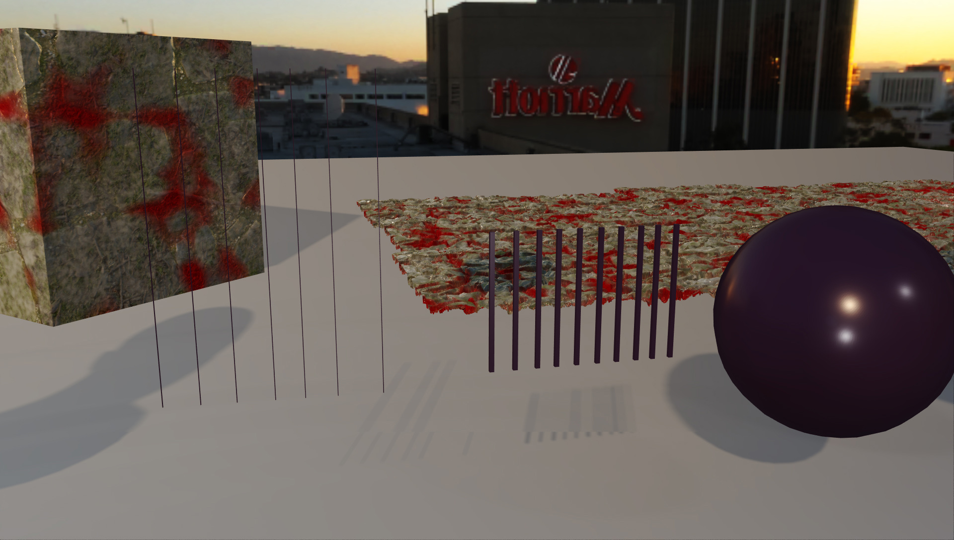
Does this work with DVM from the previous post? In short, yes. Visibility VRS does not change the fundemental structure of the GBuffer. So the single frame case “just works”. The one area that still requires more work is TAA. I adjusted the DVM accumulation formula, and it works, but it is not quite as clean in movement for small objects as the regular 1x TAA case. In order to properly tweak TAA you need to spend several months obsessing over every corner case in your content, fiddling with passes and numbers to optimize every detail. Unfortunately, I don’t have real content to test with, and it doesn’t make sense to spend several months fine-tuning the parameters of a toy engine. TAA with DVM converges when stationary and subjectively looks acceptable in motion. But it is definitely not as good as it could be, and optimizing it will have to wait for another day.
Sparse GBuffers
One side note is that the GBuffer is sparse. However, most screen-space passes require sampling nearby values in the GBuffer. So what are the options?
- Extract Full-Res: The simplest option would be to run the same pass on the GBuffer as we do on lighting. I.e. just expand it to full-res. That would have a significant bandwidth cost, but it's the easiest solution.
- Extract Half-Res: As an alternative, we could skip the full-res GBuffer, and just go to half-res. Would it be acceptable for any pass which needs neighbors to get a half res-version. Would SSAO really degrade that much if it was forced to use a half-res normal?
- Embrace Sparsity: Then again, do we actually need a full-res GBuffer? Perhaps, instead of storing a full GBuffer, we could get away with only storing a list of several nearby samples? For example, in Subsurface Scattering we generally want to randomly sample a nearby point. We don't actually care about that particular point. Rather we just want to randomly sample from a reasonable point a certain distance away without bias. So if each pixel gave us a list of 4 pixels to choose from, we could randomly choose one of those 4. It should be possible to tweak the math to do it without bias. But this would require a thorough examination of all the GBuffer passes, and most engines have a lot of them.
It seems plausible that we can do most of our screen-space passes without paying for a full-res GBuffer. Maybe a hybrid approach would be best, such as extracting world normals to full-res but leaving everything else sparse? I don’t have the answer to that question, but it seems like an interesting problem to solve.
Sample Choosing
Also worth noting is that various presentations on VRS have discussed different metrics for reducing the shading rate. In this implementation, the only inputs to determining pixel priority are the pass index, the distance to an edge, and if a pixel has no neighbors. But there are many other options. In no particular order:
- Pixels that lack detail can of course use fewer samples. Classic detection method is a Sobel filter.
- Objects in motion tend to be blurry, so we can reduce samples on pixels with large motion vectors.
- Areas under heavy transparency can reduce sample count.
- Pixels under the scene GUI certainly do not need to be rendered at full rate.
- Areas that are out-of-focus from DOF can be sampled at a lower rate as well.
- We can disable shading rate in the skybox pixels.
- Foveated Rendering in VR can significantly drop the shading rate.
I’m sure there are others. Which of those would makes sense to use? Honestly, all of them, and I still see the possibility of major wins from using these techniques. But in order to do that, it would need to be tested on a wider variety of content which was impractical for this implementation.
References
[1] Next-Generation Gaming with AMD RDNA 2 and DirectX 12 Ultimate. AMD. (https://community.amd.com/t5/blogs/next-generation-gaming-with-amd-rdna-2-and-directx-12-ultimate/ba-p/427032)
[2] Variable Rate Shading in Call of Duty: Modern Warfare. Michal Drobot. (https://research.activision.com/publications/2020-09/software-based-variable-rate-shading-in-call-of-duty–modern-war)
[3] Variable Rate Shading Tier 1 with Microsoft DirectX 12 From Theory to Practice. Marissa du Bois and John Gibson. (https://www.youtube.com/watch?v=d-qEvmVcg8I)
[4] Get Started with Variable Rate Shading on Intel Processor Graphics. Intel. (https://software.intel.com/content/www/us/en/develop/articles/getting-started-with-variable-rate-shading-on-intel-processor-graphics.html)
[5] Deferred Adaptive Compute Shading. Ian Mallet and Cem Yuksel. (https://geometrian.com/data/research/dacs/HPG2018_DeferredAdaptiveComputeShading.pdf)
[6] Efficient Adaptive Deferred Shading with Hardware Scatter Tiles. Ian Mallet, Cem Yuksel, and Larry Seiler. (https://dl.acm.org/doi/abs/10.1145/3406184)
[7] VRWorks - Variable Rate Shading (VRS). NVIDIA. (https://developer.nvidia.com/vrworks/graphics/variablerateshading)
[8] Variable Rate Shading: A scalpel in a world of sledgehammers. Jacques van Rhyn. (https://devblogs.microsoft.com/directx/variable-rate-shading-a-scalpel-in-a-world-of-sledgehammers/)
[9] Moving Gears to Tier 2 Variable Rate Shading, Jacques van Rhyn. (https://devblogs.microsoft.com/directx/gears-vrs-tier2/)
[10] A Deferred Material Rendering System. Tomasz Stachowiak. (https://onedrive.live.com/view.aspx?resid=EBE7DEDA70D06DA0!115&app=PowerPoint&authkey=!AP-pDh4IMUug6vs)
comments powered by Disqus
