Adventures in Visibility Rendering
- Part 1: Visibility Buffer Rendering with Material Graphs
- Part 2: Decoupled Visibility Multisampling
- Part 3: Software VRS with Visibility Buffer Rendering
- Part 4: Visibility TAA and Upsampling with Subsample History
Introduction
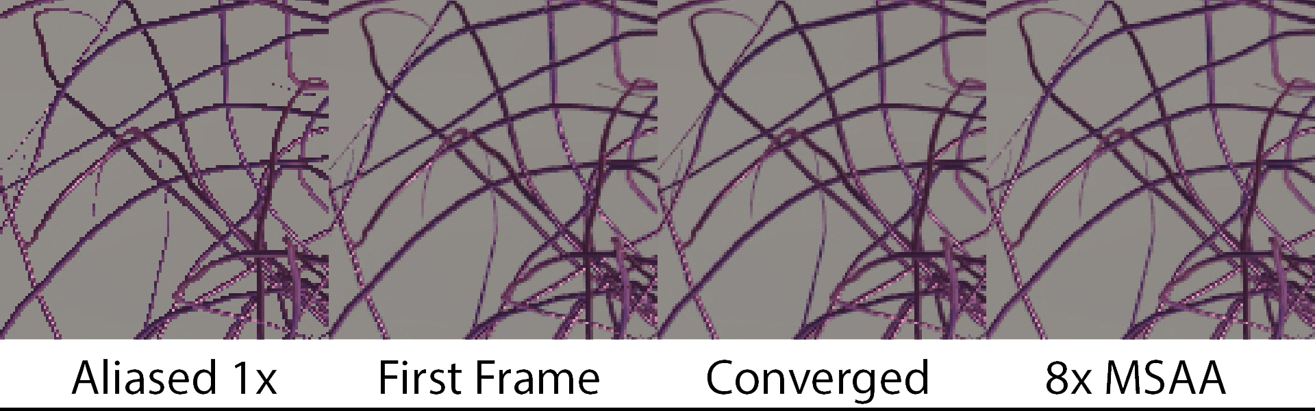
Decoupled Visibility Multisampling (DVM) is an antialiasing technique that works by decoupling the geometry and shading sample rates. Triangle visibility is rendered with 8x MSAA, but a 1x GBuffer is rendered. Most prior art that splits the geometry and shading rate starts with the assumption that shading rate should always be at least 1x, and then they try to add extra samples with as little overhead as possible. In contrast, DVM renders with a fixed rate of 4 samples per 4 pixels in a single 2x2 quad. When a given pixel needs more than one sample, instead of adding a sample, DVM switches the sample within the 2x2 quad. This approach keeps the GBuffer at a fixed size, and avoids the branches and divergent GBuffer texture fetches of other approaches. In cases where a 2x2 quad needs more than 4 samples, the approach falls back to TAA.
Standard TAA Algorithms will generally begin the first frame with an aliased image, like the one below:
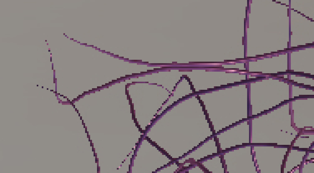
However, we’re not going to do that. Rather, we will use our 8x MSAA Visibility buffer to perform an edge-aware dilation of our samples allowing the first frame in the sequence to have anti-aliased edges.

Finally, each additional frame will refine the result using temporal information for shading, much like TAA.
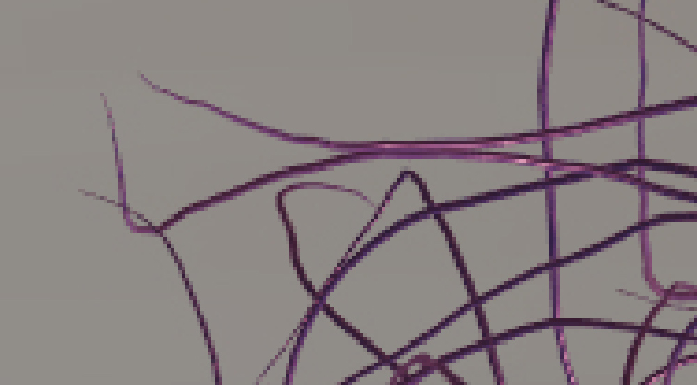
The net result is that we can achieve MSAA style edges with temporal accumulation similar to TAA.
As mentioned in the previous post, there are very interesting things you can do with Visibility rendering. And if you have not read that post, I’d highly recommend that you do before reading this one. The main point was that with Visibility rendering, the shading pass is completely decoupled from the geometry rasterization pass. And the previous post showed the benefits of that decoupling for performance, mainly in terms of quad overdraw.
Previous Post: Visibility Buffer Rendering with Material Graphs
But the much more interesting aspect of decoupling the shading pass from rasterization is that your shading rate is no longer tied to your rasterization rate. In this particular variation, we are going to render the visibility buffer at 8x MSAA. However, the shading rate will be fixed at 1x. Since the shading rate is 1x, we use a standard, regular 1x GBuffer (with a little bit of sample switching), for standard, regular shading. Then we can use a visibility buffer to dilate those samples onto geometry at a higher spatial sampling rate. Since we are exploiting the fact that visibility decouples geometry samples from shading samples, the natural name for this technique is Decoupled Visibility Multisampling (DVM).
Visual Acuity and Vernier Acuity
Before diving in, there is one other question we should address: Why do this? Why is it desirable to decouple the geometry sampling rate from the shading sampling rate?
Mathematically, aliasing happens when a signal is undersampled. There are many different types of aliasing that can happen in realtime graphics. Aliasing can happen both inside and outside of triangles. So why are triangle edges so important?
We tend to imagine that our eye is like a camera. It’s assumed that the rods and cones in our retina sense the amount of light hitting them, that image gets sent to our brains, and we see that image in our consciousness. But that’s not how it actually works. We don’t have enough bandwidth in our retinal nerve to pass all that information from our eyes to our brain. For a more complete explanation of the cells in the visual system wikiwand.com has detailed articles on Photoreceptor Cells, the Receptive Field, and Retinal Ganglion Cells.
The short version is that our retina has the well-known “Rods and Cones” that detect color and luminance. However, this information does not go straight to your brain. Rather it goes into your retinal ganglion cells, which have different receptive fields. The retinal ganglion cells accumulate information from different rods and cones and pass a compressed signal to the brain. What we “see” in our heads isn’t what the real world actually looks like. Rather, it’s an approximation pieced together from the various contrast detection algorithms in our eyes.
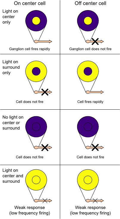
Receptive Field image from https://www.wikiwand.com/en/Receptive_field
The human eye is literally a neural network. The photoreceptors are split between cells that get excited and inhibited by light, which allows the network of retinal ganglion cells behind them to act as a contrast detection filter. Additionally, these ganglion cells fire at different rates based on the signal from the cones. If nearby retinal ganglion cells are sending a signal at a different rate, the cells behind them in the network can infer subtle details about the gradients.
As it turns out, our ability as humans to detect slight misalignment in edges is actually much higher than our ability to resolve details. The resolution at which we can detect misalignment is called Vernier Acuity, as opposed to resolving details which is called Visual Acuity. This aspect of vision has been exploited for over a century using vernier calipers. Vernier calipers rely on our ability to detect misalignment to add an extra decimal point to precise measurements.
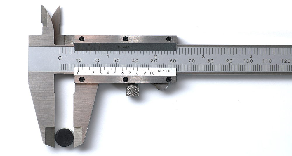
Want to see this effect on your own eyes? Take the test yourself at https://michaelbach.de/ot/lum-hyperacuity/.
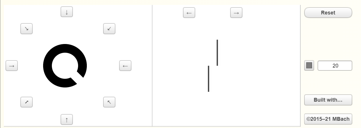
Go to this website, and I would recommend setting up your moniter 5 or 10 feet away. The empty space in the “Landolt C” is the same size as the gap between the misaligned lines. Try to get the C as small as possible. At that point, you should still be able to see the misalignment since your vernier acuity greatly exceeds your visual acuity. While that is a somewhat cursory test, the medical profession has done proper, thorough studies of vernier acuity.
According to Wikipedia, in a typical person, visual acuity has resolution of about 0.6 arc minutes, whereas vernier acuity is 0.13 arc minutes [19]. By those numbers, vernier acuity resolution is 4.6x more detailed.
So what does this mean for us in terms of computer graphics? Suppose we are rendering a triangle. We have detailed textures and shading inside the triangle. And of course, the edges of the triangle can cause aliasing as well. Our ability to resolve texture details inside will be limited the visual acuity, but our ability to see aliasing is determined by vernier acuity, which is roughly 4.6x stronger.
If we render the triangle at the resolution of visual acuity, the interior shading will look fine but the edges will be clearly aliased. However, if we render everywhere at a resolution that is high enough to exceed vernier acuity, we will be wasting cycles rendering detail that we can not see. For the ideal tradeoff between quality and performance we want to decouple the geometry and shading resolution. We want our shading resolution high enough to exceed visual acuity and the geometry resolution high enough to exceed vernier acuity.
Multisampling Anti-Aliasing (MSAA)
Multisampling performs shading and geometry at a separate resolution. As you probably know multisampling renders subsamples instead of pixels. In this case, we have a 2x2 group of pixels, with each pixel having 8 subsamples. They are split into two triangles, with orange on the left and green on the right.
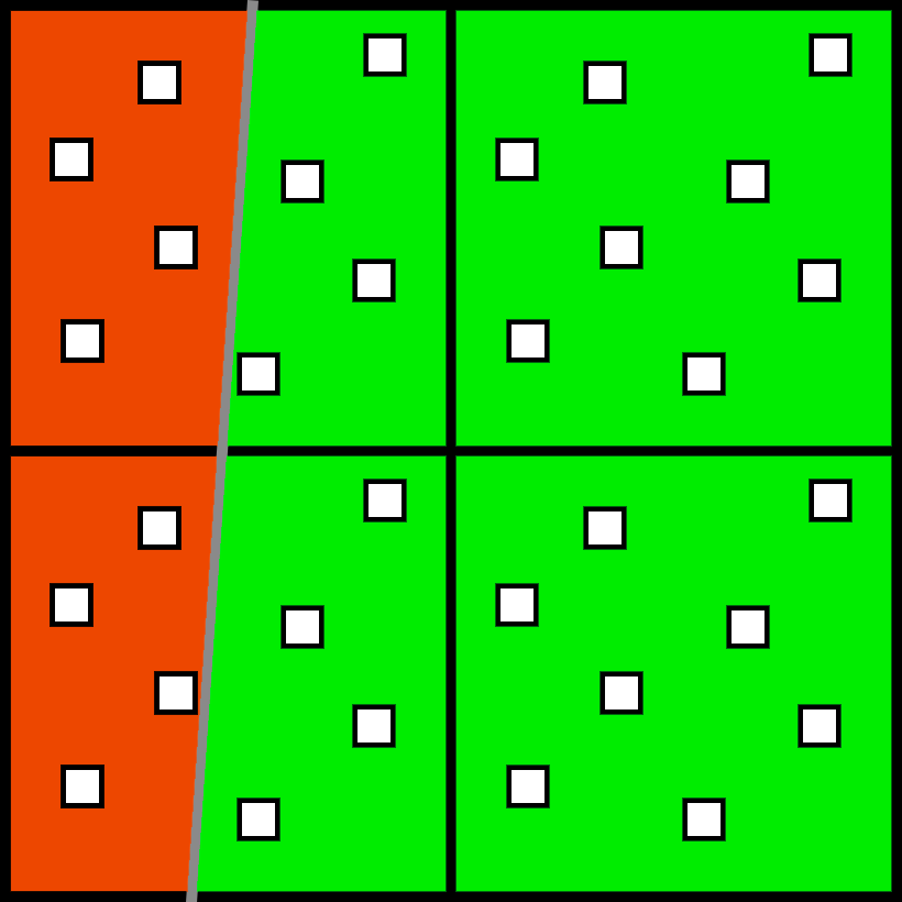
For each pixel/triangle pair, the GPU will run the pixel shader once, and then apply the same color to the other samples on the same pixel and triangle. On the upper left pixel, the GPU will calculate the orange triangle at one point, and the green triangle at another point, requiring 2 separate shader invocations. However, on the right the pixel shader will only run once.
In terms of perception, this approach is ideal. In the interior of the triangles, we have no extra work to do. And then on a triangle edge, we would run an extra sample just where we need it. We can shade our pixels at the resolution of visual acuity, and then use 4x or 8x MSAA to render our edges at the limit of vernier acuity. In the image below the left side has no AA applied, and the right side uses 8x MSAA. If you are interested, there are much more in-depth discussions of MSAA, such as is Matt Pettineo’s [13].
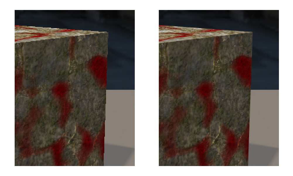
On the left side MSAA is disabled, and 8x MSAA enabled on the right.
Forward MSAA
The most obvious method to render with MSAA is Forward. But forward has general performance loss relative to Deferred and Visibility. You can read my last post discussing the impact of quad utilization, but there are other issues as well. Everything must be rendered in one giant forward pass, even though it is (usually) more efficient to split rendering into several smaller passes. There is no GBuffer for screen-space effects. And MSAA has performance issues with small triangles above and beyond the 1x sampling case.
There are several other “forward-ish” approaches for AA as well. In particular there is Jorge Jimenez’s Filmic SMAA, which ships in the Call of Duty franchise [6]. Additionally, the GPU vendors have implemented custom formats that split color and depth into different sample rates. NVIDIA developed CSAA [12] and AMD has developed EQAA [1]. Splitting the shading and geometry sample rate is definitely not a new concept!
Deferred MSAA
Another option is to render deferred, and write an MSAA GBuffer. But the trick is to only perform lighting calculations where you need it. The first approach was from Andrew Lauritzen at Intel who proposed classifying tiles to split the GBuffer lighting passes into 1x and 2x versions [8]. This approach was implemented in CryEngine3 [18] as well as a Dx11 sample from NVIDIA [11]. Matt Pettineo has a writeup of his tests as well with code you can download [14].
While those approaches can work, they usually have a fixed cost overhead in terms of memory and bandwidth to render the larger GBuffer. Anecdotally, I’ve had several backchannel discussions with teams that implemented a similar approach (like rasterizing a 2x MSAA GBuffer and only shading the edges twice). All of them removed it shortly therafter because:
- The fixed cost of even a 2x GBuffer is quite high in terms of memory and performance.
- Since many passes read from the GBuffer, the code complexity becomes a significant burden on engineering time.
In a real engine, you end up with lots and lots of corner cases where you need to read the GBuffer. Splitting that computation quickly becomes unweildly, especially if that calculation requires branches or divergent texture/memory fetches. I’ve had many variations of the same conversation with developers who implemented 2x MSAA GBuffers and then removed it in favor of TAA.
Other Approaches
There are many other creative approaches to splitting the shading rate from geometry rate. One of the earlier approaches was Surface Based Anti-Aliasing (SBAA) from Marco Salvi and Kiril Vidimče at Intel [16]. They would choose a value of N, and store at most N samples for an individual pixel using a clever multi-pass rendering approach. The DAIS paper [17] compresses visibility into a link list of visibility samples per pixel to only render as many as are needed. The Subpixel Reconstruction Anti-Aliasing (SRAA) paper [2] renders 16x depths, 1x GBuffer, and uses the depth to assist in interpolation between GBuffer samples. HRAA [5] uses the GCN rasterization modes to split coverage and shading. The Aggregate G-Buffer Anti-Aliasing paper [3] and [4] renders MSAA depth and uses Target Independent Rasterization to perform a unique depth test on different render targets to render a special Aggregate G-Buffer. Finally, the Adaptive Temporal Anti Aliasing paper [10] actually shoots rays to gather samples in-between the pixels of a 1x GBuffer.
Triangle Culling, Quad Utilization and MSAA
Another major issue when shading with MSAA is the pair of quad utilization and triangle culling, especially as triangles become very small. While the long-term goal in graphics is to have 1 pixel per triangle, that technically implies one visible triangle per pixel. If we want triangles to be one pixel wide and tall, we want the area to actually be 0.5 pixels per triangle such that half the triangles are rejected as empty. To achieve film style rendering we want pixels that are 1x1 pixel wide, not 1.4x1.4 pixels wide. We actually want 1 vertex per pixel, which means 2 triangles per pixel.
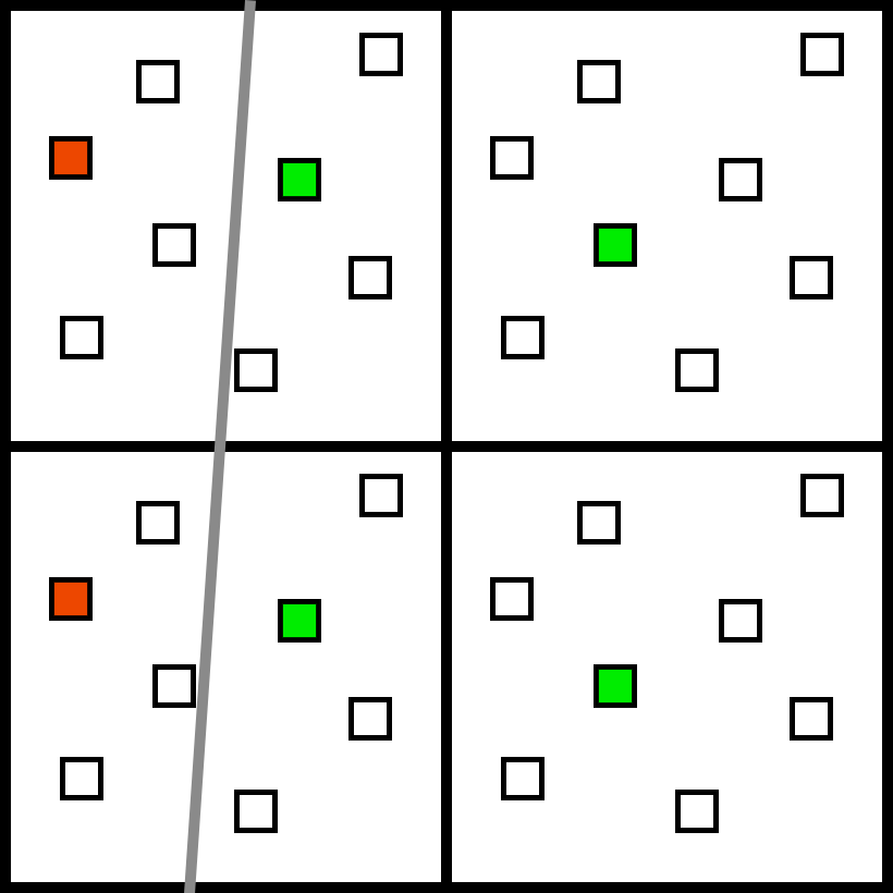
As an example, suppose we are rendering at 1080p (2 million pixels). For each pixel to hit a unique triangle, we actually need about 4 million triangles in our frame. In a standard 1x renderer, half of those triangles will be discarded. Here is a quick example, and note that the triangles which do not cover a pixel center are discarded as zero-pixel triangles. Fortunately, those triangles will not run any pixel shader invocations.
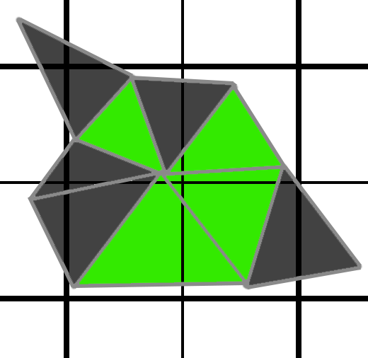
In the image above, the green triangles would have to run a shader invocation, but the greyed out pixels would not because they do not touch a pixel center. Since each triangle must run its own 2x2 pixel shader job, the GPU would render the pixel shader 4 times per pixel. But at least 4 shader invocations per pixel is as bad as it gets. However, with MSAA, it can actually get worse. In the image below, with MSAA, we now need to render the purple triangles as well.
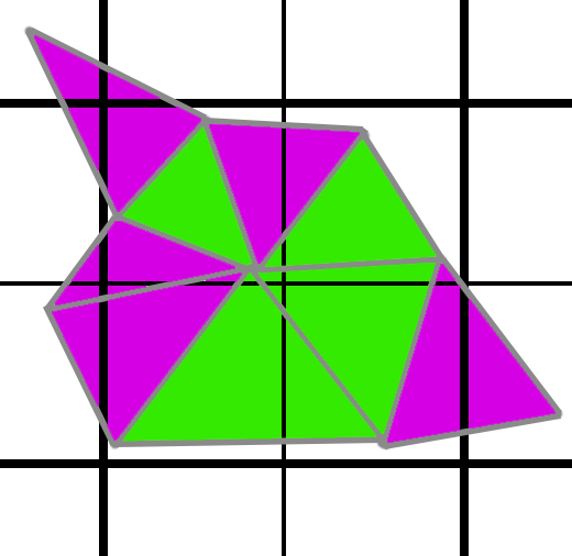
All of those triangles which did not cover any pixel centers suddenly start covering subsamples (except really tiny pixels that do not cover a single subsample). If we are rendering on average 2 triangles per pixel, we suddenly have doubled the number of pixel shader invocations we need. Instead of 4 per pixel, now we are at 8.
It still gets worse. In the grid below, the thick lines are the 2x2 quad boundaries. And if you notice, these triangles in red have subsamples on both sides of the quad boundary. While these triangles would be culled in the 1x case, they each require 4 pixel shader invocations for each side, or 8 total.
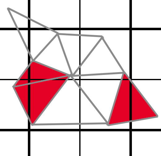
And in the even worse case? This cyan triangle up here covers 4 quad boundaries, and would require 16 total pixel shader invocations just for that one tiny little triangle.
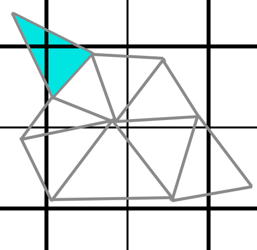
This might seem extreme, but it’s actually not. Since quad boundaries are 2 pixels wide, a pixel that is 1 pixel wide has a roughly 50% chance of touching a quad boundary. The actual chance of spawning multiple quads is a bit lower, since it would need to cover a sample on both sides of the boundary, not just touch the border. With triangles less than a pixel in size, MSAA gets absolutely wrecked by quad utilization.
If we want to get triangles down to 1 pixel in longest dimension and we want MSAA, then Forward shading is going to be rough. But before we try Visibility, we should also look at the most common anti-aliasing solution: TAA.
Temporal Antialiasing
To start off, here is a simple scene of a few long, thin cubes (like thin rods). The original image with no anti-aliasing looks like this.
Long, thin cubes with no Anti-Alisasing
With MSAA, we can fix this issue quite effectively.
Long, thin cubes with 8x MSAA
Due to the cost of MSAA, the most common approach for achieving cleaner edges in realtime is Temporal Anti-Aliasing (TAA). For a thorough discussion of prior art regarding Temporal Antialiasing, I’d recommend the paper from Lei Yang, Shiqiu Liu, and Marco Salvi [20]. While there are many variations, most implementations follow the outline of Timothy Lottes’s paper [9], Brian Karis’s presentation [7], and Marco Salvi’s presentation [15]. For this post, I’m using a standard TAA approach with 8 samples and the standard 8x multisampling locations (N Rooks instead of Halton). Also, for this implementation I’m performing color clamping in RGB space.
While details vary among implementations, the key ideas are:
- Jittered Projection Matrix
- Reprojection of the previous frame
- Color clamp/variance check to reduce ghosting.
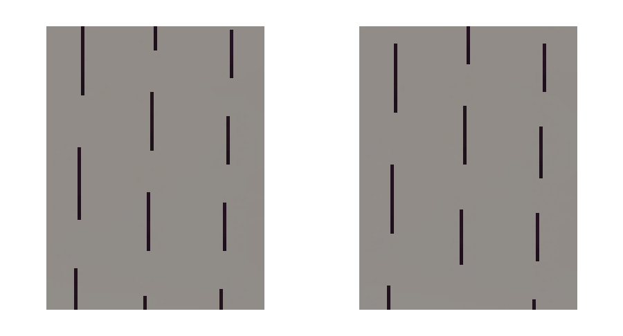
Rather than rendering 8x samples in a single frame, the idea is to render 1x sample each frame, but jitter the projection matrix so that after 8 frames, you have a sample from all 8 positions. Here is a simple shot from my toy engine showing two of the raw original frames. Note that the jaggies shift from one frame to the next due to the different subpixel offset. Obviously, they are quite aliased.
Then we can accumulate and over time we converge to the following image:
If nothing moves, then in theory the results are equivalent to supersampling. The edges are clean and look similar to MSAA/supersampling. The interiors of triangles tend to have less aliasing since TAA can help fix issues like speckles in hot specular highlights. It can also look softer than MSAA since it will clamp the peaks and valleys in the signal due to the color clamp.
While the edges look great if nothing moves, the obvious problem is that in games, things tend to move. You can see it in the typical situations like camera moves, but the most problematic areas tend to be deformable objects like grass. And even though TAA is made by 8 sequential frames, it doesn’t actually converge in 8 frames. In TAA, if a pixel moves too far, it has to reject the pixel history and start with a jagged, aliased image. Then it gets refined by using a fraction of the weight of each new frame. Most implementations seem to have a value in the range of 5% to 10%. We’ll call this value T.
As an example, if your T value is 10%, after the first frame, you will retain 90% of your original 1x frame. This process continues, so after N frames that original frame still counts for pow(1-T,N) of your final image. Below is a quick table for how much influence the original frame has after N frames have passed.
| 8 | 15 | 30 | 45 | 60 | |
|---|---|---|---|---|---|
| T=0.10 | 43.0% | 20.6% | 4.2% | 0.87% | 0.18% |
| T=0.05 | 66.3% | 46.3% | 21.5% | 9.9% | 4.6% |
Obviously, higher values of T will converge faster than low values, but the tradeoff is increased flickering. The short answer is that there is no perfect solution, and tradeoffs have to be made. If you are at T=0.1, you’ll see quite a bit of flicker. If the object is stationary or moving slowly then TAA works very well. However strong movements will invalidate the history at the edge, and TAA will fail if the history is being invalidated faster than TAA can converge. And as we all know, objects can move quite a distance in 30 to 60 frames.
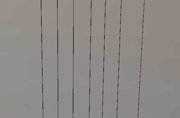
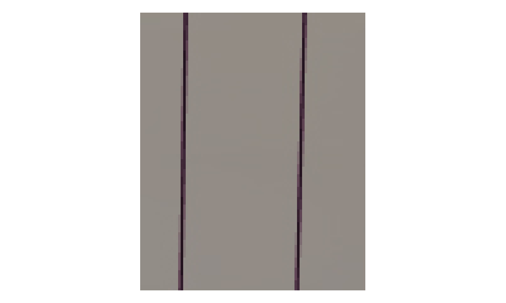
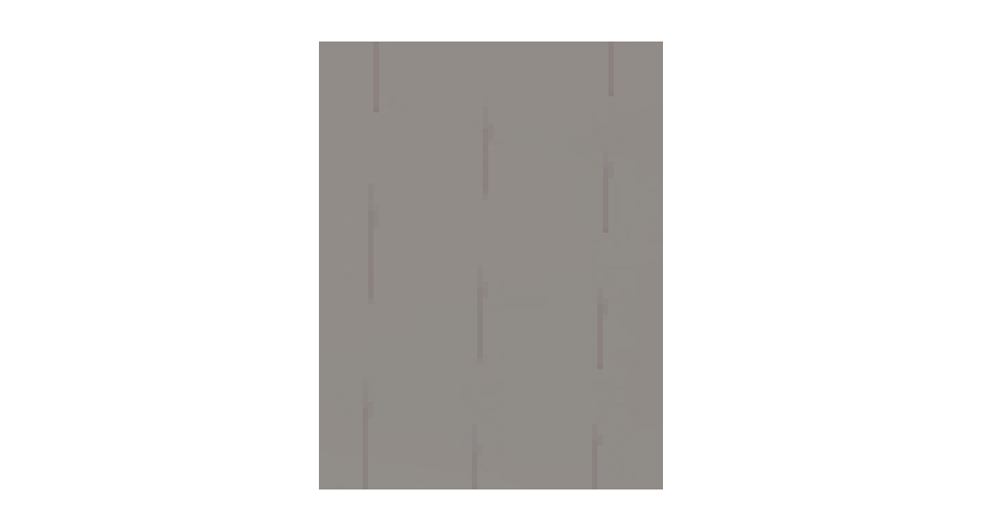
We also have another major issue with TAA: Thin objects. Now let’s look at the same image, but move the camera farther away. Here is what two of our jittered images look like before any TAA is applied.
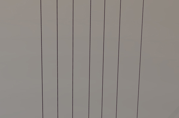
And here is the final result:
So, why does this happen? Think about the sequence of three frames.
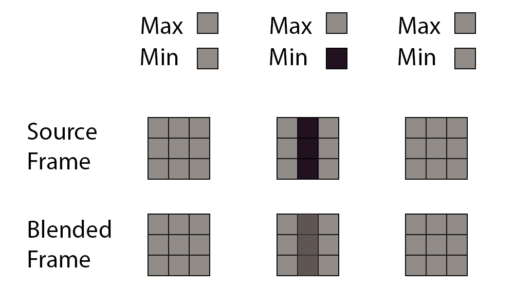
In the first frame, the patch of all pixels is grey, and naturally the min/max color box is grey as well. In the next frame, a thin object goes through the patch and will lerp with the original image using T as the weight. The problem happens in the third frame. We have another patch of all grey pixels, the min and max are grey, and the previous frame is clamped out.
At a glance it might seem like the solution is to incorporate more information, such as store the variance of the pixel. The problem is that sometimes thin objects like this are stationary, and sometimes they move. For example, if you have a thin wire swinging in the wind you would want the clamp to keep it from ghosting. But if it is stationary, you would want to avoid the clamp and keep it in the accumulated history. Unfortunately, you don’t know if the wire has actually moved until 8 frames later, so you have to make an imperfect guess. It’s a tradeoff between flickering and ghosting, and there is no perfect answer.
As the object becomes less than one pixel in width, it seems to vanish. TAA handles this case by color clamping, and as a result the image “disappears”. In addition to thin objects like wires, you can also see this effect in real games on faceted edges, like the trim on buildings. For reference, here is the MSAA8 image which is effectively the reference solution:
The primary advantage of TAA is the simplicity for the rest of the pipeline. You just render everything at 1x and TAA fixes the rest. It works very well if you have objects more than a pixel wide that have minimal movement. But it breaks down when you have too much movement or objects thinner than a pixel. Otherwise the common solution is MSAA.
Decoupled Visibility Multisampling
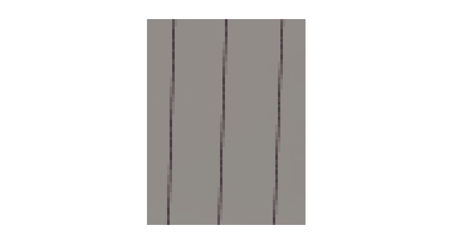
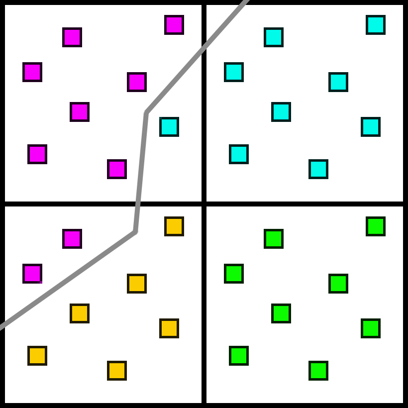
To fix these problems, let’s try something a little different. Suppose we render triangle visibility for a scene at 8x MSAA. Here is a little 2x2 quad, and the grey path is the material edge from several triangles. The subsamples would each have information on which material they point to. In this case, two different materials touch this 2x2 quad.
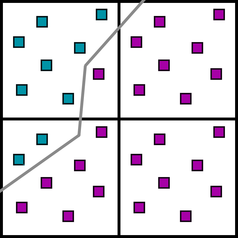
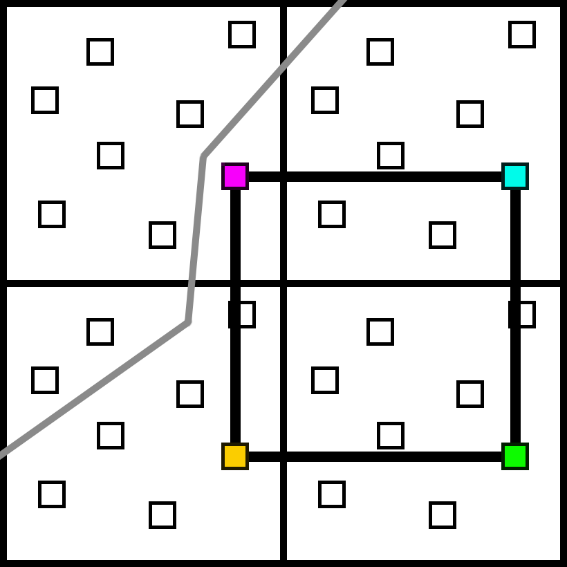
However, instead of jittering a projection matrix and rendering at 1x, let’s just extract the 1x shading samples from our 8x visibility buffer. We could actually do the same algorithm as TAA. Instead of rendering with a jittered projection matrix, we can just choose the samples from the visibility buffer that correspond to those same positions. And from here, we could render everything normally just like a 1x buffer.
However, we have information that a TAA algorithm does not. In particular, TAA does not know anything about the samples off the jitter pattern. They could have moved from the previous frame or they could be in the same spot. However, with a full visibility buffer we know exactly which material they belong to, so we can expand the influence of our samples in the same pixel.
We have several subsamples that are not filled in though, as they do not have a sample on the same pixel to use data from. In the case of MSAA, these empty pixels would be on separate triangles, and the pixel shader would evaluate an additional time. But we can get a good approximation by choosing another sample on the quad which has the same material.
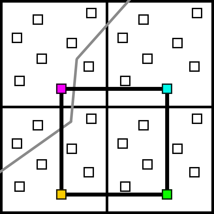
The benefits are pretty obvious. Using visibility information, we can achieve the same edge quality as MSAA8 as long as we are willing to relax our restrictions on where the colors come from. MSAA guarantees that every sample will come from a centroid that is on the same triangle and the same pixel. Whereas in this case we are relaxing our restriction to be the same material (not triangle) on the same 2x2 quad (not pixel).
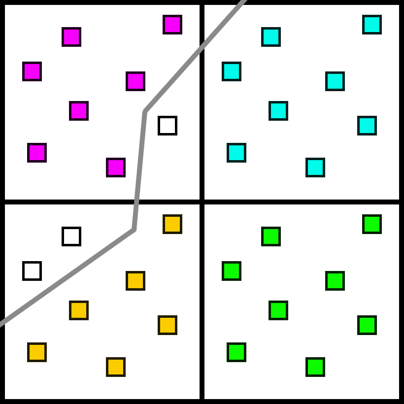
But not all situations are handled so easily. A few frames later, we will end up at this case:
If we dilate the samples, we still have unknown subsamples. Since all 4 chosen samples were from the same material, we do not have any similar samples to choose from in the 2x2 quad.
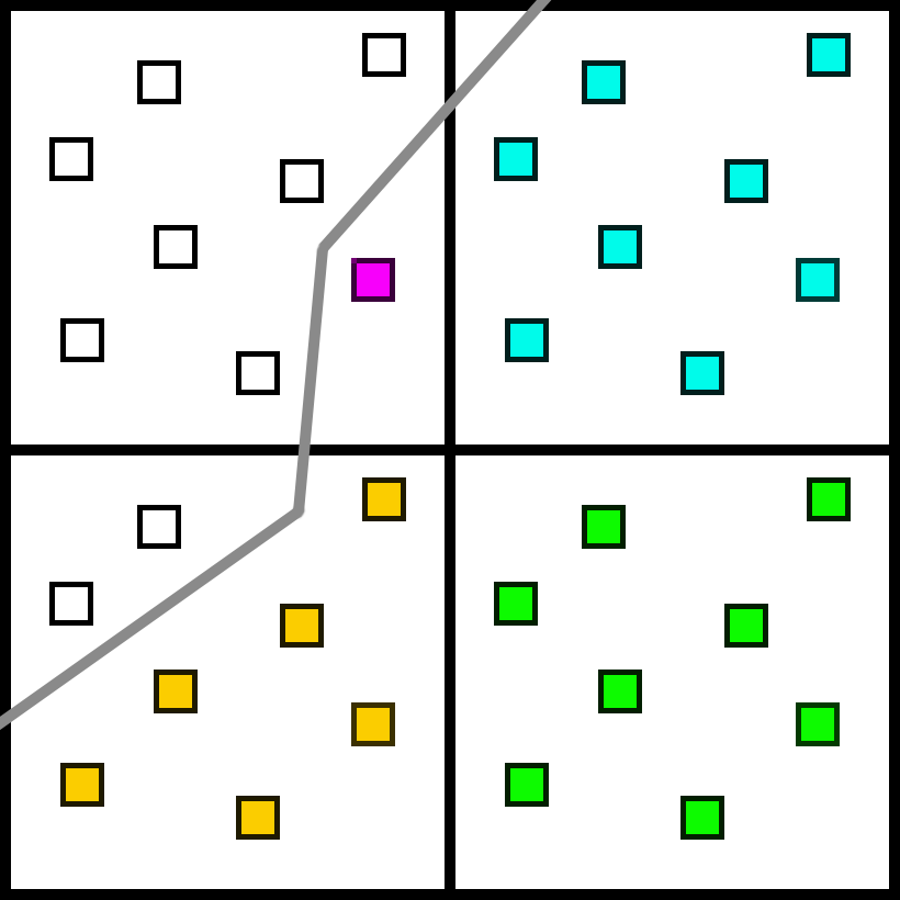
The most obvious and accurate solution would be to add a new sample.
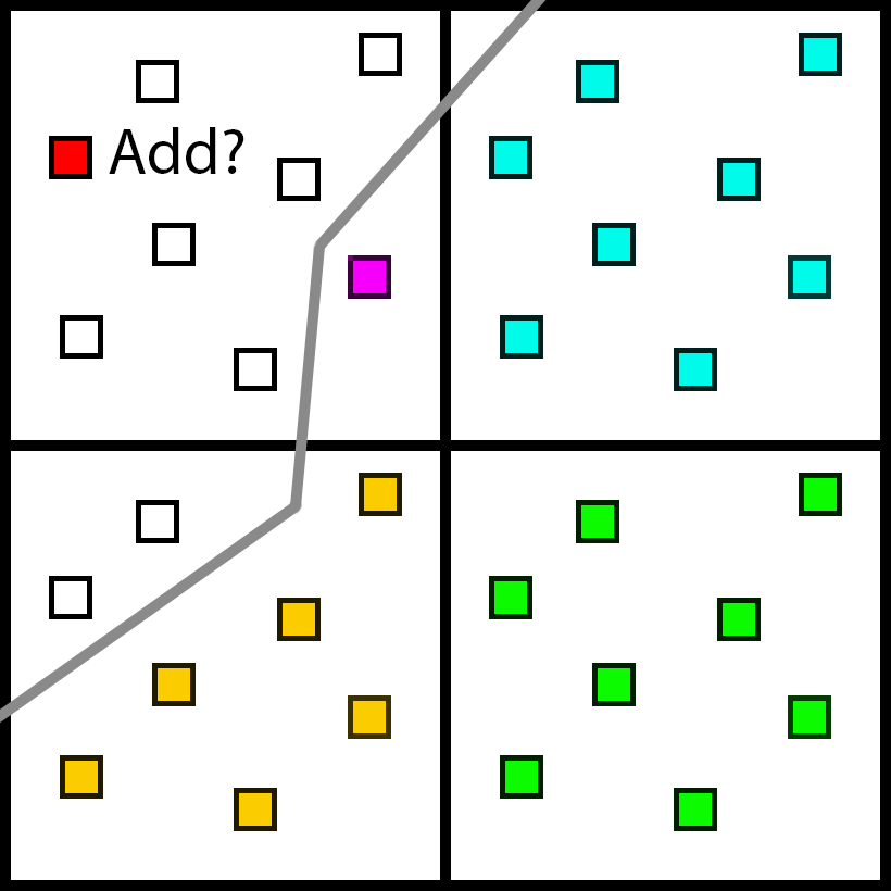
There would be a cost for adding the sample, and it would not drastically change the computation needed. It would only increase the total number of samples by a small percentage. But it adds a huge amount of subtle complexity to the renderer. Any time we need to read the GBuffer, we would need to do some kind of branch, and potentially fetch data from a non-cache-friendly location. Various screen-space passes need the GBuffer. Various materials need the GBuffer. Adding a divergent cost to every single pass is a pretty big deal, even if the actual number of samples added is small.
This approach is very similar in spirit to several previous approaches. The closest direct comparison is Surface Based Anti-Aliasing from Marco Salvi and Kiril Vidimče [16]. However the SRAA [2], ATAA [10], and DAIS [17] papers include very similar concepts as well. Still, it would be much preferred to keep the GBuffer exactly at 1x, even if it means a reasonable degradation in quality compared to a more accurate solution that adds samples.
So, instead of adding samples, why don’t we try switching the samples?
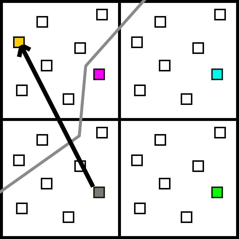
We can disable the bottom left sample, and enable a new one on the upper left in its place. Now we have at least one sample for each of the two materials in this quad. Using that sample might seem like a strange choice, though. Wouldn’t this sample make more sense, since it is closer and on the same pixel?
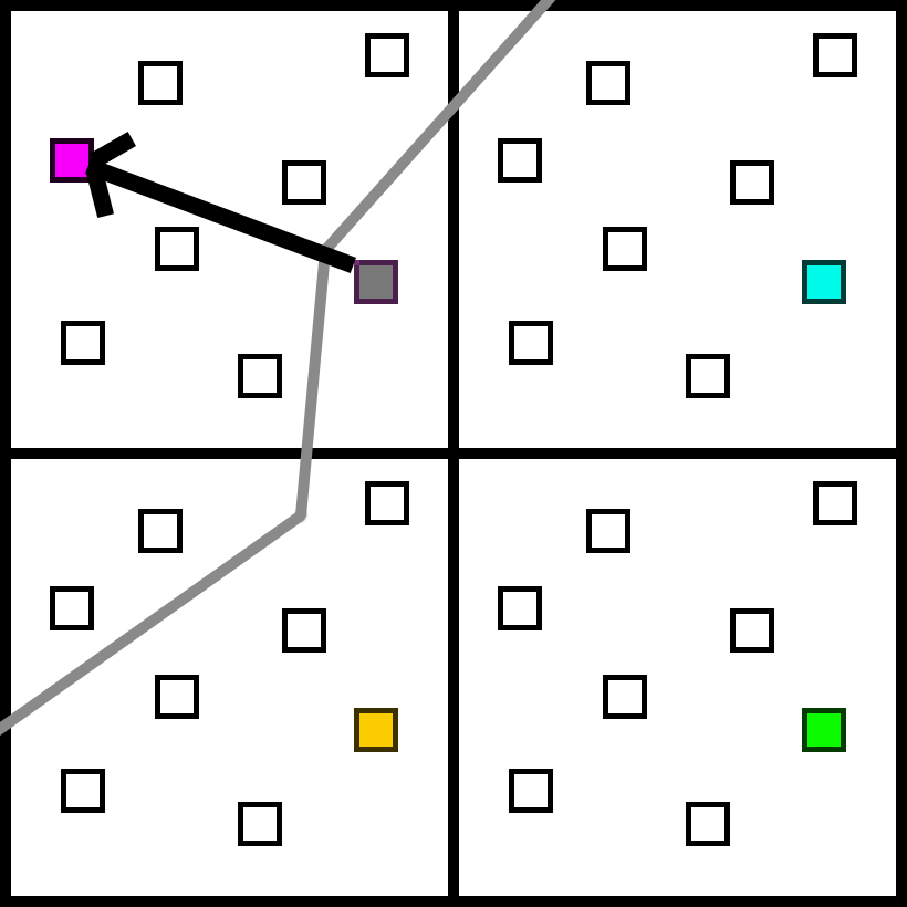
The reason is starvation. Ideally, we want every sample to have the same chance of being used to avoid biasing the final image. However, if we were to prioritize samples from the same pixel, that pixel would always be switched out and never contribute. So when we need to switch a sample, we randomly pick from the available samples instead of prioritizing samples from the same pixel. This approach will bias the image as certain samples have more weight than others, but it’s the best we can do.
You might notice that the samples in the bottom left are chosen randomly, as opposed to using the nearest pixel. Once again, the goal is to minimize bias. There will be plenty of bias of course, but we can at least try to reduce it as much as possible.
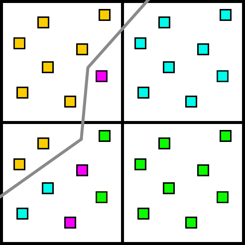
Finally, what do we do if we have too many materials?
In this case, we try to fall back to TAA as gracefully as possible. We will choose 4, and some subsamples will not be covered. In practice, the number of 2x2 quads that touch 5 unique materials is quite low, so it’s acceptable for the algorithm to become slightly blurry in that case as long as it does not flicker or cause a strong visual artifact.
The data structure is quite simple. For each sample, we need a triangle visibility ID just like the regular visibility algorithm. Since a 2x2 quad at 8x MSAA has exactly 32 subsamples, each sample has a 32 bit mask to store the coverage. Also, since samples can be switched, we need to store a 5-bit index to keep track of which of the 32 possible locations to use for lighting calculations. So the total additional storage per-pixel is a 32bit uint for visibility ID (triangle and draw call ID), a 32bit uint for the coverage mask, and 5 bit index to know this sample’s subpixel location.
The visibility uint32 is stored in the exact same way as the previous post. We can treat the GBuffer as a standard, 1x GBuffer. There are no extra branches or data reads when performing GBuffer lighting calculations. We just need to be a little more careful when determining the screen-space (x,y) position.
Finally, how do we perform the resolve? For each pixel, we need to read the 4 visibility ids and the 4 masks. Each 2x2 block shares the same values, so each pixel only needs to read 1 visibility id and mask. Then the 4 samples can be shared using SM 6.0 intrinsics without actually using shared memory. Since the data is per 2x2 quad, it also should work if we need to read the GBuffer data in either a compute or a rasterization pass. The easiest way to explain it is with a source code snippet.
float3 myColor  = TexFetch();
uint   myMask   = MaskFetch();
float3 sumColor = 0;

uint numMarked0 = countbits(myMask & baseMask);
sumColor += float(numMarked0) * myColor;

uint numMarked1 = countbits(QuadReadAcrossX(myMask) & baseMask);
sumColor += float(numMarked1) * QuadReadAcrossX(myColor);

uint numMarked2 = countbits(QuadReadAcrossY(myMask) & baseMask);
sumColor += float(numMarked2) * QuadReadAcrossY(myColor);

uint numMarked3 = countbits(QuadReadAcrossDiagonal(myMask) & baseMask);
sumColor += float(numMarked3) * QuadReadAcrossDiagonal(myColor);

uint totalMarked = numMarked0 + numMarked1 + numMarked2 + numMarked3;
float3 avgColor = sumColor * rcp(float(totalMarked));
This shader also required changing the standard TAA algorithm in a few ways. Typically, a TAA algorithm would calculate the color clamp based on the 3x3 neighborhood. However, I was able to get better results for determining the clamp for each pixel in the 2x2 grid by doing a 3x3 search and only using other pixels that share the same draw call ID. Then the min and max are interpolated in the same way as the regular resolve.
float3 myMin    = MinOfNeighborsWithSameDrawCallId();
float3 myMax    = MaxOfNeighborsWithSameDrawCallId();
float3 sumMin = 0;
float3 sumMax = 0;

sumMin += float(numMarked0) * myMin;
sumMax += float(numMarked0) * myMax;

sumMin += float(numMarked1) * QuadReadAcrossX(myMin);
sumMax += float(numMarked1) * QuadReadAcrossX(myMax);

sumMin += float(numMarked2) * QuadReadAcrossY(myMin);
sumMax += float(numMarked2) * QuadReadAcrossY(myMax);

sumMin += float(numMarked3) * QuadReadAcrossDiagonal(myMin);
sumMax += float(numMarked3) * QuadReadAcrossDiagonal(myMax);

float3 avgMin = sumMin * rcp(float(totalMarked));
float3 avgMax = sumMax * rcp(float(totalMarked));
This approach gives you a tighter box that is weighted by coverage. One lingering issue was that in some cases, thin objects would flicker. This problem occurs on a surface that has a sharp change in lighting within a single pixel, such as faceted edges. In some cases, the jittered position is in the bright pixels, other times in the dark pixels. As a somewhat hacky solution, I faded out the color clamp in cases where camera movement is less than 0.05 pixels, but a better solution would be to clamp based on per-pixel variance.
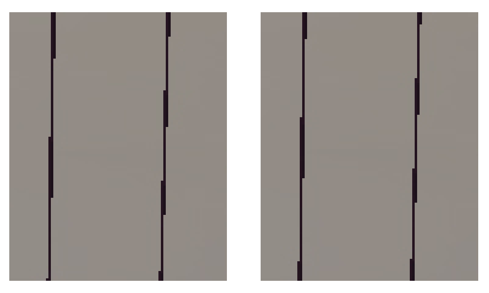
Here are some results with the thin cubes from before. The left side is an aliased frame (what the first frame of TAA would look like), and the right side is the first frame with DVM.
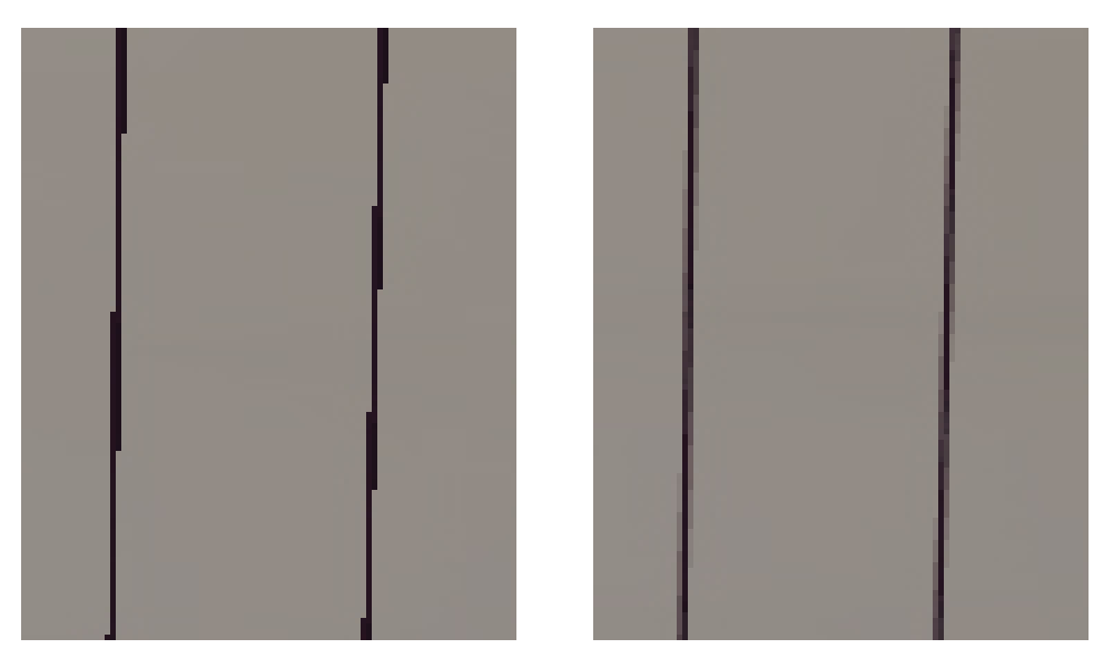
Regular 1x image on left, and the DVM image on the right.
And here is the comparison between the temporally accumulated DVM image and the MSAA image.
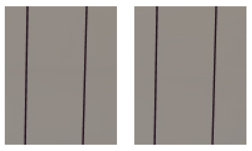
DVM on left, 8xMSAA on right.
Here is the same thing for the most difficult case, after zooming out where the thin object is less than a pixel wide. This is the case where TAA fails to converge to the correct result due to the color clamp.
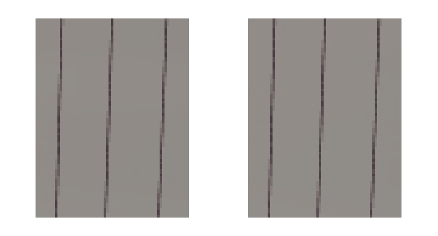
DVM on left, 8xMSAA on right.
Of course, this should not be a surprise. If there are 4 or less unique materials in a 2x2 quad, DVM is using the exact same coverage mask as MSAA for each material. The only difference is that MSAA is ensuring a unique color sample for each unique triangle per pixel, whereas DVM is only averaging one color sample per pixel and using jitter to temporally accumulate the shading results (like TAA).
Performance
For testing performance, I’ll use the same scenes as in the previous blog post. Although I made a few changes to the methodology. In the previous post, the shadows were very inefficient as the dense meshes are naively rendered. So for this test, the shadows were tweaked so that if nothing changes from the previous frame, then the depth maps are reused from the previous frame. Since these tests are all with a static camera, we do not have any shadow depth rendering in these tests.
The results below show timing numbers of several different rendering paths.
- Forward: Regular forward rendering with TAA.
- Msaa 2x/4x/8x: Regular forward with MSAA, and no TAA since they perform an MSAA resolve.
- Deferred: Deferred shading with TAA.
- Visibility: Visibility rendering (1x) with TAA.
- DVM: Decoupled Visibility MSAA, with 8x samples.
Here is a short discussion of the passes:
- PrePass: The Prepass performs a depth-only prepass for the Forward, Deferred, and MSAA renders. For Visibility, it renders 1x Depth and 1x VisibilityID, whereas for DVM it renders 8x Depth and 8x VisibilityID.
- Materials: Forward and MSAA have this pass combined with lighting, since a single shader performs material evaluation and lighting. Deferred performs a regular GBuffer rasterization pass. Visibility and DVM take an identical code path which evaluates the material samples in an indirect compute shader.
- Lighting: Forward and MSAA skip this pass (as it is combined with Material). Deferred performs a full screen lighting pass in a compute shader. Visibility and DVM run lighting as an indirect compute shader, skipping sky pixels.
- Motion: The rendering paths have very different algorithms for calculating motion vectors. Forward and Deferred calculate static motion vectors from reprojecting the depth to the previous view, and then render moving geometry a second time. The MSAA path calculates a 1x depth buffer, and then proceeds along the same path as Forward/Deferred. Visibility and DVM perform motion vector calculations in a compute shader. The MSAA versions are slower due to the extra depth resolve.
- Resolve/TAA: This category accounts for the Resolve and TAA time. Forward, Deferred, and Visibility perform regular TAA. MSAA applies a simple resolve in Reinhard space, and DVM applies the more complicated resolve algorithm.
- VisUtil: This number includes all the major Visibility and DVM passes. It includes analyzing the Visibility ID buffer and radix sorting the materials. It also includes the DVM analysis pass which chooses and switches the samples.
- Other: This category includes everything else. There are several miscellaneous barriers, a debug GUI pass, HDR tonemapping, and several extra copies. Note that the MSAA passes are about 0.1ms longer than the other render paths because of redundant copies. Some of the passes use render target textures, and others use buffers. If this was a real, production renderer those would be optimized out. But to keep the code simple, there are a few extra copies which are included in this number.
- Shadows: Note that there is no shadow depth pass. When nothing is moving, shadows are reused from the previous frame. So shadow depth maps are not being rasterized in these tests.
- Total: Total is full render time. Note that Other is determined from Total minus all the other passes.
Low-Density Triangles:
| PrePass | Material | Lighting | VisUtil | Motion | Resolve/TAA | Other | Total | |
|---|---|---|---|---|---|---|---|---|
| Forward | 0.020 | 1.600 | 0.093 | 0.177 | 0.353 | 2.243 | ||
| Msaa 2x | 0.038 | 1.615 | 0.092 | 0.075 | 0.443 | 2.263 | ||
| Msaa 4x | 0.072 | 1.648 | 0.092 | 0.079 | 0.439 | 2.330 | ||
| Msaa 8x | 0.124 | 1.686 | 0.109 | 0.251 | 0.439 | 2.609 | ||
| Deferred | 0.019 | 1.06 | 0.753 | 0.093 | 0.178 | 0.363 | 2.466 | |
| Visibility | 0.043 | 1.239 | 0.797 | 0.347 | 0.103 | 0.176 | 0.332 | 3.109 |
| DVM | 0.224 | 1.250 | 0.795 | 0.719 | 0.118 | 0.418 | 0.373 | 3.989 |
Medium-Density Triangles (about 10 pixels per triangle):
| PrePass | Material | Lighting | VisUtil | Motion | Resolve/TAA | Other | Total | |
|---|---|---|---|---|---|---|---|---|
| Forward | 0.132 | 3.881 | 0.093 | 0.176 | 0.354 | 4.636 | ||
| Msaa 2x | 0.211 | 4.705 | 0.110 | 0.083 | 0.463 | 5.572 | ||
| Msaa 4x | 0.361 | 5.649 | 0.146 | 0.121 | 0.464 | 6.741 | ||
| Msaa 8x | 0.560 | 6.382 | 0.205 | 0.252 | 0.460 | 7.859 | ||
| Deferred | 0.132 | 2.942 | 0.764 | 0.094 | 0.178 | 0.363 | 4.473 | |
| Visibility | 0.158 | 1.614 | 0.826 | 0.466 | 0.104 | 0.175 | 0.228 | 3.645 |
| DVM | 0.626 | 1.618 | 0.827 | 0.921 | 0.119 | 0.420 | 0.261 | 4.882 |
High-Density Triangles (about 1 pixel per triangle):
| PrePass | Material | Lighting | VisUtil | Motion | Resolve/TAA | Other | Total | |
|---|---|---|---|---|---|---|---|---|
| Forward | 1.004 | 8.987 | 0.094 | 0.176 | 0.391 | 10.652 | ||
| Msaa 2x | 0.874 | 15.262 | 0.112 | 0.099 | 0.457 | 16.804 | ||
| Msaa 4x | 0.949 | 23.261 | 0.148 | 0.157 | 0.468 | 24.983 | ||
| Msaa 8x | 1.487 | 27.211 | 0.235 | 0.257 | 0.463 | 29.653 | ||
| Deferred | 1.006 | 4.640 | 0.772 | 0.093 | 0.221 | 0.371 | 7.103 | |
| Visibility | 1.156 | 1.696 | 0.836 | 0.294 | 0.101 | 0.175 | 0.404 | 4.742 |
| DVM | 1.530 | 1.745 | 0.836 | 0.965 | 0.118 | 0.421 | 0.259 | 5.968 |
All timing numbers are in milliseconds. The numbers are pretty similar to the previous post, which makes sense since it is using the same rendering algorithm. The biggest change from the previous numbers is that the shadow pass has been removed. It does look like the shadow pass was overlapping with the other passes more than I had previously thought, which was changing the numbers. For example, in my original tests, with low density triangles, the Deferred Material pass and the Visibility Material pass were the exact same length. That was likely caused by overlap from the shadow depth pass, and now the Visibility Material pass is 17% longer, which makes sense for the extra vertex interpolation and partial derivative calculations.
The DVM pass takes about 1.2ms more than Visibility, although that number is closer to 0.9 in the low triangle density case. GPUs optimize the memory layout of MSAA to minimize the fetching cost when triangles are not dense, which explains the discrepancy. Spending 1.2ms to ensure that your first frame has clean edges instead of waiting for TAA to converge seems like a pretty good tradeoff. Of course, it would be more than that on older hardware making the technique less compelling. Also, those passes are unoptimized, so I’m sure there is room for improvement.
And finally, the cost for MSAA with Forward rendering is absolutely brutal. Here is a table of just the Forward shader pass from the Forward and MSAA render paths:
| Low | Medium | High | |
|---|---|---|---|
| Forward | 1.600 | 3.881 | 8.987 |
| Msaa 2x | 1.615 | 4.705 | 15.262 |
| Msaa 4x | 1.648 | 5.649 | 23.261 |
| Msaa 8x | 1.686 | 6.382 | 27.211 |
Just…ouch. When the triangles are not dense, MSAA 8x is great. The cost only increases by a tiny 5% compared to 1x. But switching to dense triangles takes us from 1.686ms to 27.211ms. When triangles get small, performance with MSAA falls off a cliff.
And here is the same table, divided by the Forward/Low pass (i.e. dividing all numbers by 1.600). This gives us the cost of the pass relative to the baseline, best-case Forward cost.
| Low | Medium | High | |
|---|---|---|---|
| Forward | 1.00 | 2.43 | 5.62 |
| Msaa 2x | 1.01 | 2.94 | 9.54 |
| Msaa 4x | 1.03 | 3.53 | 14.54 |
| Msaa 8x | 1.05 | 3.99 | 17.01 |
Due to quad utilization, we would expect the Forward pass with 1-pixel triangles to be 4x longer than the low density triangle case. But the actual number is 5.62, which implies that we are paying a 1.41x cost per shader invocation (possibly due to increased primitive rasterization cost) multiplied in with the 4x shader invocations from poor quad utilization. At high density, the 2x, 4x, and 8x scale by an additional 1.70x, 2.59x, and 3.03x on top of 1x for the same triangle count.
But when you run the numbers, it makes sense. For 8x at high density compared to 1x at low density, we are paying:
- 1.41x in higher GPU cost per shader invocation, which is due to bandwidth, interpolators, etc.
- 4x for worst-case quad utilization.
- 3.03x for triangles that touch a sample but not a pixel center. These pixels are rendered in the MSAA case but culled as 0 pixel triangles in the 1x case.
Multiply those together and you get 17x. And while 8x is extreme, the 2x and 4x MSAA cases are still quite rough. Finally, here is one more table. Given the Visibility numbers, we can estimate how much it would cost if we switched DVM to brute force supersampling:
| High Triangle Density Forward | Estimated Brute Force Supersampling | |
|---|---|---|
| Forward | 8.987 | 2.581 |
| Msaa 2x | 15.262 | 5.162 |
| Msaa 4x | 23.261 | 10.324 |
| Msaa 8x | 27.211 | 20.648 |
Note that the DVM pass can calculate Material and Lighting in 2.581ms. In theory, the quad utilization of forward MSAA is bad enough that we really could brute force render supersampled visibility at less cost. Those numbers assume linear scaling of time as the number of samples increases.
Looking at the numbers, the use case that jumps out at me is VR. In particular, the usual game tricks to fake detail in materials (like normal maps) don’t work in VR because your eye can see through the illusion. The best practice is to really push the triangle count and reduce your material complexity. Unfortunately pushing the triangle count is the worst thing you can do for performance with Forward and MSAA. Still, proper parallax is compelling enough to make it worth the very high cost. With such poor quad utilization, trading Forward/MSAA for Visibility with DVM or even Visibility supersampling starts to look compelling.
Future Work
There are a few pretty obvious next steps. The major performance win would be optimizing the passes. These shaders have not been optimized properly.
The big quality improvement would be to add samples instead of switching them. In general, I have come to really like having a list of samples and 32bit masks per 2x2 quad. In the initial implementation, I had made a completely arbitrary number of samples per quad, but the performance just wasn’t there which was why I redesigned the algorithm to use exactly 4 samples per quad. However, I’m quite optimistic about a hybrid approach to use the first 4 samples as is, and then have an option to add a few extra samples where they add the most visual impact.
With an MSAA visibility buffer, rendering extra samples is trivial. The material compute shader runs on a flat list of visibility samples, so it is very easy to add several extra samples to the list at sharp edges. Previous papers have done great work on determining which samples to add, so incorporating that work is an obvious direction to go. The hard part is efficiently incorporating these samples into all the GBuffer passes in a more complex engine.
References
[1] EQAA Modes for AMD 6900 Series Graphics Cards. AMD. (https://developer.amd.com/wordpress/media/2012/10/EQAA%2520Modes%2520for%2520AMD%2520HD%25206900%2520Series%2520Cards.pdf)
[2] Subpixel Reconstruction Antialiasing for Deferred Shading. Matthäus G. Chajdas, Morgan McGuire, and David Luebke. (https://research.nvidia.com/sites/default/files/pubs/2011-02_Subpixel-Reconstruction-Antialiasing/I3D11.pdf)
[3] Aggregate G-Buffer Anti-Aliasing (Slides). Cyril Crassin, Morgan McGuire, Kayvon Fatahalian, and Aaron Lefohn. (https://casual-effects.com/research/Crassin2015Aggregate/Crassin2015Aggregate-presentation.pdf)
[4] Aggregate G-Buffer Anti-Aliasing -Extended Version-. Cyril Crassin, Morgan McGuire, Kayvon Fatahalian, and Aaron Lefohn. (https://graphics.stanford.edu/~kayvonf/papers/agaa_tvcg2016.pdf)
[5] Hybrid Reconstruction Anti Aliasing. Michal Drobot. (http://advances.realtimerendering.com/s2014/drobot/HRAA_notes_final.pdf)
[6] Dynamic Temporal Antialiasing and Upsampling in Call of Duty. Jorge Jimenez. (https://www.activision.com/cdn/research/Dynamic_Temporal_Antialiasing_and_Upsampling_in_Call_of_Duty_v4.pdf)
[7] High Quality Temporal Supersampling. Brian Karis. (http://advances.realtimerendering.com/s2014/#_HIGH-QUALITY_TEMPORAL_SUPERSAMPLING)
[8] Deferred Rendering for Current and Future Rendering Pipelines. Andrew Lauritzen. (https://software.intel.com/content/dam/develop/external/us/en/documents/lauritzen-deferred-shading-siggraph-2010-181241.pdf)
[9] TSSAA: Temporal supersamping AA. Timothy Lottes. (http://timothylottes.blogspot.com/2011/04/tssaatemporal-super-sampling-aa.html)
[10] Adaptive Temporal Antialiasing. Adam Marrs, Josef Spjut, Holger Gruen, Rahul Sathe, and Morgan McGuire. (https://research.nvidia.com/sites/default/files/pubs/2018-08_Adaptive-Temporal-Antialiasing/adaptive-temporal-antialiasing-preprint.pdf)
[11] Antialiased Deferred Rendering. NVIDIA. (https://docs.nvidia.com/gameworks/content/gameworkslibrary/graphicssamples/d3d_samples/antialiaseddeferredrendering.htm)
[12] Coverage Sampled Antialiasing. NVIDIA. (https://developer.download.nvidia.com/SDK/9.5/Samples/DEMOS/Direct3D9/src/CSAATutorial/docs/CSAATutorial.pdf)
[13] A quick Overview of MSAA. Matt Pettineo. (https://therealmjp.github.io/posts/msaa-overview/)
[14] Bindless Texturing for Deferred Rendering and Decals. Matt Pettineo. (https://therealmjp.github.io/posts/bindless-texturing-for-deferred-rendering-and-decals/)
[15] An excursion in temporal supersampling. Marco Salvi. (https://developer.download.nvidia.com/gameworks/events/GDC2016/msalvi_temporal_supersampling.pdf)
[16] Surface Based Anti-Aliasing. Marco Salvi and Kiril Vidimče. (https://software.intel.com/content/dam/develop/external/us/en/documents/43579-SBAA.pdf)
[17] Deferred Attribute Interpolation for Memory-Efficient Deferred Shading. Cristoph Schied and Carsten Dachsbacher. (http://cg.ivd.kit.edu/publications/2015/dais/DAIS.pdf)
[18] CryEngine3 Graphics Gems. Tiago Sousa. (https://advances.realtimerendering.com/s2013/Sousa_Graphics_Gems_CryENGINE3.pptx)
[19] Visual Acuity. Wikipedia. (https://en.wikipedia.org/wiki/Visual_acuity)
[20] A Survey of Temporal Antialiasing Techniques. Lei Yang, Shiqiu Liu, and Marco Salvi. (http://behindthepixels.io/assets/files/TemporalAA.pdf)
comments powered by Disqus