Adventures in Visibility Rendering
- Part 1: Visibility Buffer Rendering with Material Graphs
- Part 2: Decoupled Visibility Multisampling
- Part 3: Software VRS with Visibility Buffer Rendering
- Part 4: Visibility TAA and Upsampling with Subsample History
Introduction
The last year or so has been strange for everyone. Each of us has been dealing with covid quarantine in our own way, and in my case I’ve been coding. As you likely know, small triangles are ineffcient on GPUs for a variety of reasons, including low quad utilization. Since a Visibility Buffer is, in theory, more resilient than Deferred for cases with poor quad utilization, I’ve had this hunch that a Visibility Buffer renderer would be able to get better performance than a classic Deferred renderer. With a bit of free time on my hands, I put together a Dx12 toy engine for testing this theory.
Overview and Prior Art
The idea of a visibility buffer is pretty simple. During a first pass you render a “Visibility Buffer” which stores the object and triangle IDs in a single value, usually a packed U32. Then that triangle/object ID is all you need to fetch any parameters that you need.
The initial major paper was from Christopher Burns and Warren Hunt at Intel [3]. In addition to coining the term “Visibility Buffer”, they were the first reference I could find to storing a triangle ID and reconstructing the interpolated vertex data. To handle multiple materials, they split the screen into tiles and classified the pixels inside them. Then they would render a single draw call per material only covering the tiles that touch the needed pixels. A Visibility buffer has also been used to optimize rendering in other ways, such as Christoph Schied and Carsten Dachsbacher [12] who approached the problem as a multisampling compression algorithm. Wolfgang Engel from ConfettiFX has demonstrated a visibility buffer [5], forgoing arbitrary material graphs but using bindless textures. Their approach treats materials as one ubershader with arbitrary texture access. They also provide source code under a permissive license so I’d highly recommend taking a look if you are interested [4].
The most recent work of course is Nanite in Unreal 5, from Epic Games. They approach the problem differently from the past. While I don’t have any secrets to tell you, the high-level approach is publicly known. Instead of using a Visibility Buffer as a replacement for a GBuffer, they are using a Visibility Buffer as an optimization to create a GBuffer more efficiently. In particular, GPU rasterizers have performance inefficiencies with small triangles, so Nanite uses a custom rasterizer to bypass these bottlenecks as you can see in their overview videos [7]. Note that you can jump to 1:00:45 for the quick discussion on triangle sizes. The UE5 visibility rasterizer is a Nanite-only rasterizer, so other objects go through the standard Deferred path.
In theory, with Visibility rendering there is no need for a GBuffer. If you need the normal, you can always fetch it directly from the vertex parameters. And if you need it again, you can fetch it again. But in practice, material graphs are already quite long, and they are getting longer every year. If all we needed was direct lighting, then we could do without a GBuffer. But since we need values like the normal multiple times per frame (direct lighting, screen-space reflections, ambient probes, etc), storing material outputs in a GBuffer seems like the way to go.
In the variation proposed here, the Visibility Buffer will be used to generate the GBuffer, and we will use it for all triangles. We’re also going to do this with arbitrary material graphs, which means calculating our own analytic partial derivatives. In doing these tests, there are several questions I am trying to find the answer to:
- Can we efficiently calculate analytic partial derivatives with material graphs?
- In other words, is this approach viable, at all? If we can't calculate analytic partial derivatives, this approach is a non-starter.
- For very high triangle counts (1 pixel per triangle), is the Visibility approach faster?
- Is this approach faster for future workloads? If we want to hit film quality, eventually we need all triangles down to 1 pixel in size. Backgrounds, characters, grass, props, everything.
- What about more typical triangle sizes (5-10 pixels per triangle)? Is the Visibility approach faster there too?
- Is this approach faster for current AAA game workloads?
Turns out, in the tests below the answer to all three questions is: Yes! But with the caveat that this is a toy engine and not a real AAA engine.
Forward/Deferred/Visibility Overview
First, we should do a quick overview of Forward, Deferred, and Visibility rendering. In forward rendering, you are calculating everything in a single pixel shader, which will look something like this.
struct Interpolators; // the position, normal, uvs, etc.
struct BrdfData; // normal mapped normal, albedo color, roughness, metalness, etc.
struct LightData; // the output lighting data, usually just a float3

// Pass 0: Render all meshes, output final light color
LightData MainPS(Interpolators interp)
{
  BrdfData  brdfData  = MaterialEval(interp);
  LightData lightData = LightingEval(brdfData);
  return lightData;
}
Fundamentally, every physically based Forward shader starts with the hidden step that isn’t in the code: Interpolating vertices. The hardware interpolates the vertex data, and it magically passes the interpolated vertex data in for you. Of course, hardware isn’t magical, but that step does happen before the pixel shader code begins executing. In the next step, the MaterialEval() function will take the interpolated values (like UVs, normals, and tangents) to perform math and texture lookups to calculate surface material params. These typically include the normal-mapped normal, the base color, etc. In the final step, it evaluates every light for those parameters and outputs the resulting color.
However, the more common approach for rendering in games these days is Deferred, using a GBuffer, which renders in two passes.
// Pass 0: Render all meshes, output material data.
BrdfData MaterialPS(Interpolators interp)
{
  BrdfData  brdfData  = MaterialEval(interp);
  return brdfData;
}

// Pass 1: Compute shader (or large quad) to calculate lighting.
LightData LightingCS(float2 screenPos)
{
  BrdfData  brdfData  = FetchMaterial(screenPos);
  LightData lightData = LightingEval(brdfData);
  return lightData;
}
The Deferred approach uses the same basic steps as Forward. However the lighting data is evaluated in a separate pass, either a full-screen quad, or a compute shader. The benefits are:
- The big advantage is that the lighting function is guaranteed to run exactly once per pixel. When rasterizing geometry MaterialPS() may run more than once per pixel, but LightingCS() is guaranteed to only run once.
- When the MaterialEval() and LightingEval() functions are in the same shader, they get compiled with the worst case register allocation for both, whereas when they are split one pass can use fewer registers than the other (and achieve better occupancy).
- With the deferred approach, we have a GBuffer which can be used for other effects, such as Screen-space Reflections, SSGI, SSAO, and Subsurface Scattering.
The obvious drawback is that Deferred increases the amount of bandwidth used. In general the screen-space effects you can do and the improved shader performance greatly outweigh the bandwidth and memory cost. Of course, all that goes out the window if you absolutely need MSAA, but that is a whole other discussion.
Visibility rendering takes a very different approach. Instead of rasterizing the lighting color (like Forward) or the GBuffer data (like Deferred), visibility rasterizes only the ID for the triangle and draw call. We could also store a barycentric co-ordinate or derivatives, but we are going to use a single triangle ID.
// Pass 0: Rasterize all meshes, just output thin visibility
U32 VisibilityPS(U32 drawCallId, U32 triangleId)
{
  return (drawCallId << NUM_TRIANGLE_BITS) | triangleId;
}

// Pass 1: In a CS convert from triangle ID to BRDF data
BrdfData MaterialCS(float2 screenPos)
{
  U32 drawCallId = FetchVisibility() >> NUM_TRIANGLE_BITS;
  U32 triangleId = FetchVisibility() &      TRIANGLE_MASK;

  Interpolators interp    = FetchInterpolators(drawCallId, triangleId);
  BrdfData      brdfData  = MaterialEval(interp);
  return brdfData;
}

// Pass 2: In a CS, fetch BRDF data and calculate lighting
LightData LightingCS(float2 screenPos)
{
  BrdfData      brdfData  = FetchMaterial(screenPos);
  LightData     lightData = LightingEval(brdfData);
  return lightData;
}
Note that we have a separate pass for the Material and Lighting steps, which is different from most prior art [3,13]. Most previous papers have performed both steps together in order to reduce GBuffer bandwidth. But given the complexity of material shaders, my perspective is that we need a GBuffer. Material shaders can be very long, but they are long for legitimate tech-art reasons. Material shaders made by artists can be inefficient (maybe a slight understatement). But even when they are a complete mess, there is usually a good, valid reason for the effect the material is trying to achieve, even if that effect is not achieved in the most performant way. My personal view is that long material graphs are here to stay, they are going to be expensive, and we need to figure out the most efficient way to handle it.
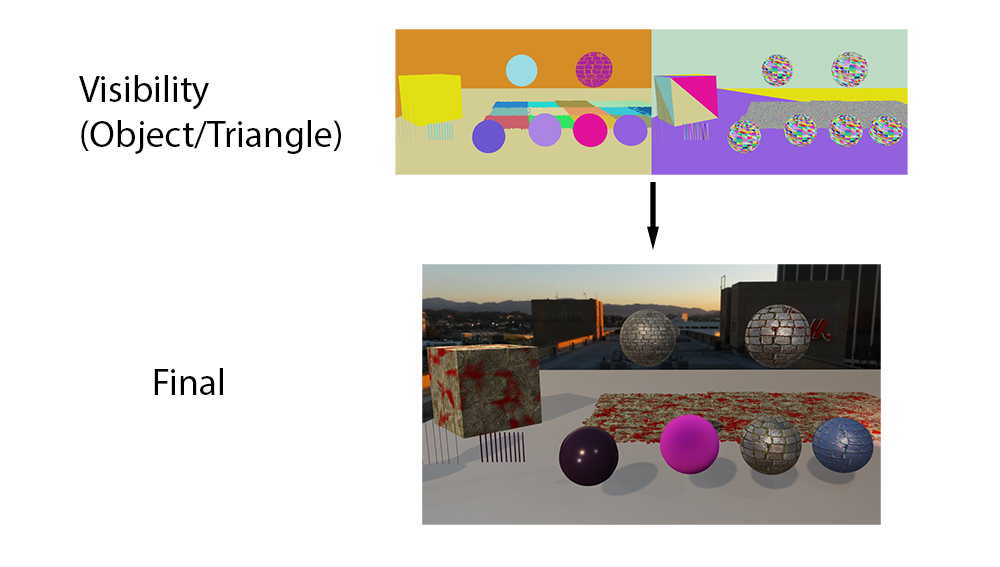
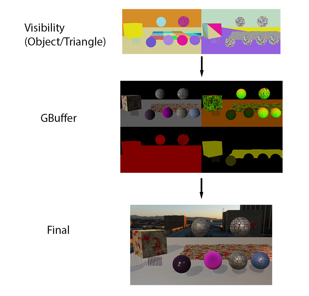
In this case though, how do we handle multiple materials, and in particular material graphs? We’ll use the flow diagrammed below.
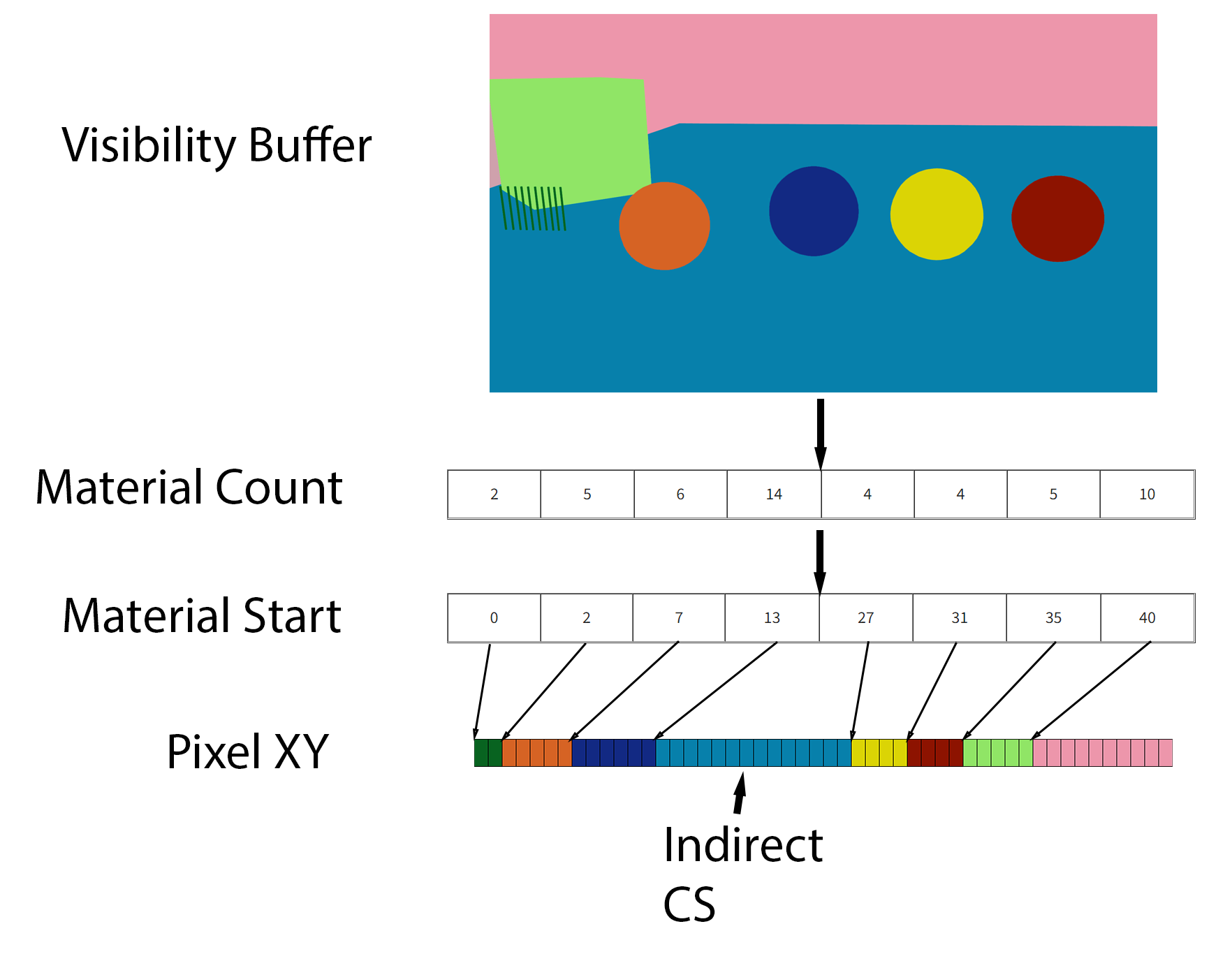
- As a first step, we render the full screen visibility buffer.
- Go through each pixel, and calculate the number of pixels used for each material. Store the result in the Material Count buffer.
- Perform a prefix sum to figure out the Material Start.
- Run another pass through the visibility buffer, storing the XY position of each pixel in the appropriate position in the Pixel XY buffer. Note that the Pixel XY buffer has the same number of elements as the Visibility Buffer.
- For each material, run an indirect compute shader to calculate the GBuffer data.
That is how the passes are ordered, and it allows us to render multiple material graphs with different generated HLSL code. However there is one more issue to address when calculating GBuffer data: Partial Derivatives.
Hardware Partial Derivatives
If you have written a pixel shader, at some point you have surely written a line to read from a texture. Something like this:
Sampler2D sampler;
Texture2D texture;
...
float2 uv = SomeUv();
float4 value = texture.Sample(sampler,uv);
When you run this code, the GPU will figure out the optimal mipmap level to read from and filter the data for you. But how does it figure out the correct mipmap level?
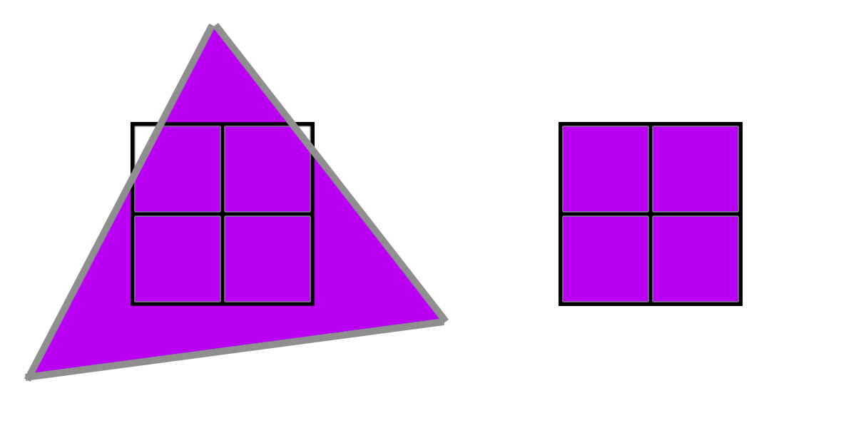
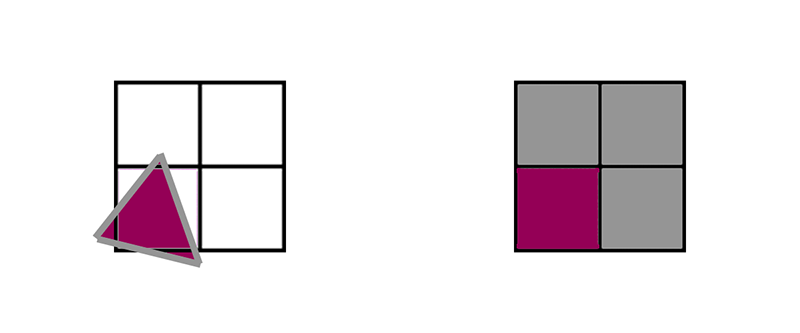
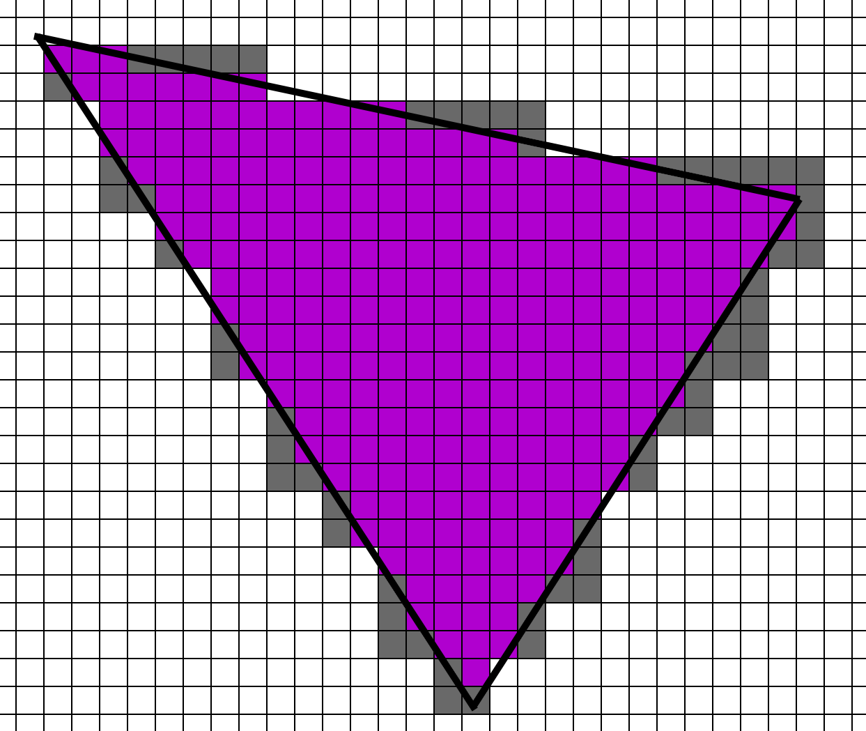
The key is that pixel shaders don’t run on single pixels. Rather, they run on 2x2 groups of pixels, called a quad. In the purple example below, the triangle covers all 4 pixels, all 4 pixels run the same shader in lockstep, and during the texture read the GPU will compare the 4 uv values to determine the mipmap level. The GPU can estimate the partial derivative w.r.t. x by subtracting the left pixels from the right pixels and the partial derivative w.r.t. y by subtracting the top from the bottom. Then it can determine the proper level from the log2 of that difference. This approach is called finite differences.
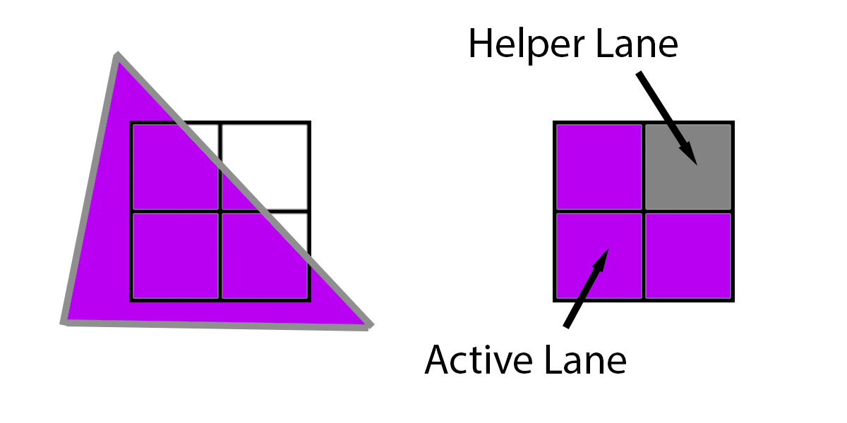
However, what happens if a triangle does not cover all 4 pixels, such as this triangle below which only covers 3? In that case, the GPU will extrapolate the triangle onto that missing pixel, and run it like normal. The 3 pixels that are actually running are called “Active Lanes” and the 1 pixel which is only running to provide derivatives to the other three is a “Helper Lane.”
For more information, see the HLSL Shader Model 6.0 wave intrinsics doc [9]. In fact, there are intrinsics to pass data around between with other pixels in the same 2x2 quad. However, what happens if multiple triangles overlap the same 2x2 quad?
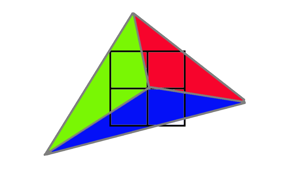
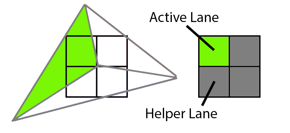
In this sample, 3 different triangles cover sample centers in the 2x2 grid. First up, the green triangle covers the upper left corner. To render this, the GPU would render the upper left pixel as an active lane and the other three would be shaded as helper lanes, providing texture derivatives to the one active lane.
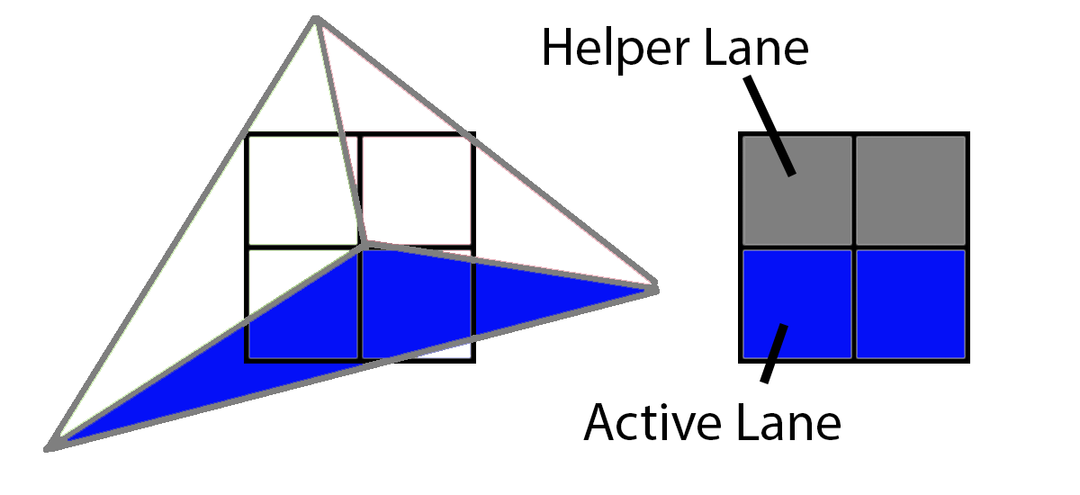
Next up, the blue triangle would have 2 active lanes and 2 helper lanes.
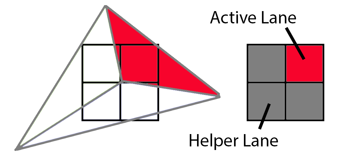
And finally, the red triangle would have 1 active lane and 3 helper lanes.
When we have 1 triangle that covers all 4 pixels in a quad, the pixel shader workload looks like this:

But when we have 3 triangles that cover the 4 pixels in a quad, the pixel shader workload looks like this:
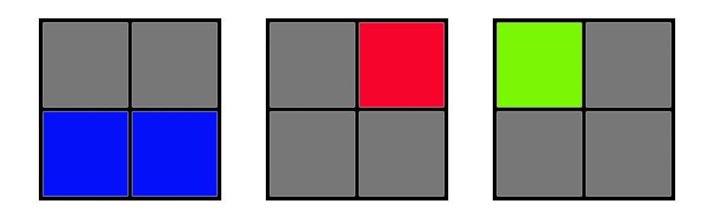
If we have 3 triangles covering the same 2x2 quad, then we actually have 3 times as much pixel shader work to do relative to a single triangle covering all 4 pixels. This ratio of active lanes divided by total lanes is Quad Utilization. The purple quad has 100% quad utilization but the workload of these three triangles has 33% quad utilization. And what is the main factor that affects quad utilization? Triangle size.
Quad Utilization Efficiency
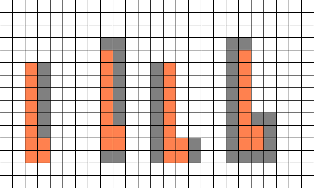
Given this, suppose that we are rendering only 1 pixel triangles. Even with no overdraw, each 2x2 quad would have 1 active lane and 3 helper lanes.
If we were to render the entire scene with 1 pixel triangles, we would have to execute each pixel shader 4 times per pixel, instead of just one. The Forward and Deferred Material shaders would run 4 times for every pixel, whereas the Deferred Lighting and Visibility Material and Lighting passes would only run once per pixel.
Shader function invocations per pixel for 1-pixel sized triangles:
| Material | Lighting | |
|---|---|---|
| Forward | 4x | |
| Deferred | 4x | 1x |
| Visibility | 1x | 1x |
Going to the other extreme, what happens if we have big, large triangles? In that case it’s much simpler. The number of helper lanes will be a small percentage of the overall pixels rendered, and for the purposes of this post we can call it incidental. The pixels shaders are running about once per pixel.
Approximate shader function invocations per pixel for large triangles:
| Material | Lighting | |
|---|---|---|
| Forward | 1x | |
| Deferred | 1x | 1x |
| Visibility | 1x | 1x |
Those are the extremes, but what happens in the middle? The middle is more complicated. The conventional wisdom is to aim for about 10 pixels per triangle. What is the quad utilization of a 10 pixel triangle? It will vary by the shape, but let’s try a few and find out. We’ll start with the simplest 10 pixel triangle.
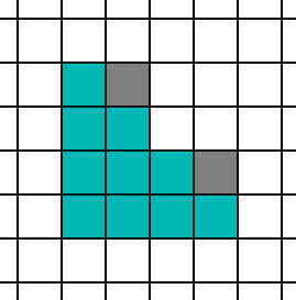
At a glance, it looks really good, as there are 10 active lanes and only 2 helper lanes. However, there are 4 possible ways that this triangle can align to the 2x2 grid.
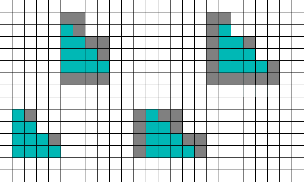
If you do the counting, on average you end up with 9 helper lanes to the 10 active lanes. Next, let’s try one that is a little longer and thinner.
With this shape, we have on average 11 helper lanes to the 10 active lanes. Here is the worst-case shape:
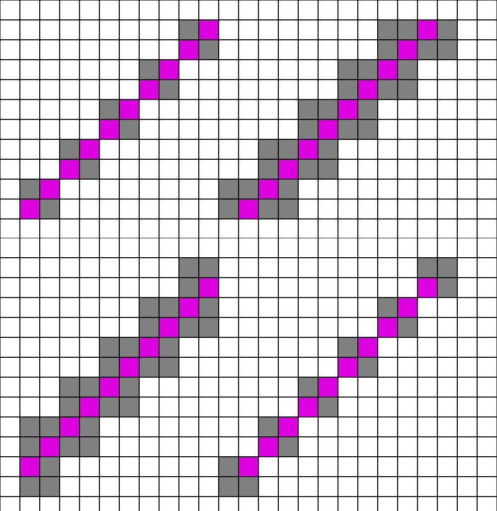
If I counted that one correctly, it’s 21 helper lanes to 10 active lanes (ouch). Now, that’s an extreme case as a triangle would have to be perfectly aligned to cause a shape like that. As a reasonable estimate, if we say that the first (cyan) and second (orange) triangles happen equally, and the third (purple) never happens, we will hit 50% quad utilization. In other words, the Forward and Deferred Material passes will run about 2x per pixel. Once again, Deferred Lighting and Visibility Material and Lighting will run once per pixel.
Approximate shader function invocations per pixel for 10 pixel triangles:
| Material | Lighting | |
|---|---|---|
| Forward | 2x | |
| Deferred | 2x | 1x |
| Visibility | 1x | 1x |
At a glance, Visibility rendering suddenly looks very compelling compared to Deferred. With 10 pixel sized triangles the Deferred Material pass has to run 2x as many times as the Visibility Material pass, and it turns into 4x if triangles are one pixel. However, the Visibility pass has extra work to do.
Interpolation and Analytic Partial Derivatives
Whereas the Deferred approach relies on the hardware to pass the interpolators to the pixel shader, we have to fetch and interpolate this data ourselves. The first step is fetching data, which is relatively straightforward. Note that you can gain significant wins by packing the data aggressively, but for this test the data is stored as 32bit floats for simplicity. g_dcElemData is the draw call element data, which is a StructuredBuffer that contains important per-instance data, such as where the vertex buffer starts.
uint3 FetchTriangleIndices(uint dcElemIndex, uint primId)
{
  TriangleIndecis ret = (TriangleIndecis)0;
  uint startIndex = g_dcElemData[dcElemIndex].m_visStart_index_pos_geo_materialId.x;
  return g_visIndexBuffer.Load3(startIndex + 3 * 4 * primId);
}

TrianglePos FetchTrianglePos(uint dcElemIndex, TriangleIndecis triIndices)
{
  uint startPos = g_dcElemData[dcElemIndex].m_visStart_index_pos_geo_materialId.y;

  TrianglePos triPos = (TrianglePos)0;
  triPos.m_pos0.xyz = asfloat(g_visPosBuffer.Load3(startPos + 12 * triIndices.m_idx0));
  triPos.m_pos1.xyz = asfloat(g_visPosBuffer.Load3(startPos + 12 * triIndices.m_idx1));
  triPos.m_pos2.xyz = asfloat(g_visPosBuffer.Load3(startPos + 12 * triIndices.m_idx2));
  return triPos;
}
It’s not a lot of instructions, but what hurts performance is stalls waiting for the data. Fetching UVs and normal data is much the same so we’ll skip listing it here. The next step is to calculate the barycentric co-ordinate. The DAIS paper [12] has a very handy formula in Appendix A, and the ConfettiFX code is a very useful reference as well [4].
struct BarycentricDeriv
{
  float3 m_lambda;
  float3 m_ddx;
  float3 m_ddy;
};

BarycentricDeriv CalcFullBary(float4 pt0, float4 pt1, float4 pt2, float2 pixelNdc, float2 winSize)
{
  BarycentricDeriv ret = (BarycentricDeriv)0;

  float3 invW = rcp(float3(pt0.w, pt1.w, pt2.w));

  float2 ndc0 = pt0.xy * invW.x;
  float2 ndc1 = pt1.xy * invW.y;
  float2 ndc2 = pt2.xy * invW.z;

  float invDet = rcp(determinant(float2x2(ndc2 - ndc1, ndc0 - ndc1)));
  ret.m_ddx = float3(ndc1.y - ndc2.y, ndc2.y - ndc0.y, ndc0.y - ndc1.y) * invDet * invW;
  ret.m_ddy = float3(ndc2.x - ndc1.x, ndc0.x - ndc2.x, ndc1.x - ndc0.x) * invDet * invW;
  float ddxSum = dot(ret.m_ddx, float3(1,1,1));
  float ddySum = dot(ret.m_ddy, float3(1,1,1));

  float2 deltaVec = pixelNdc - ndc0;
  float interpInvW = invW.x + deltaVec.x*ddxSum + deltaVec.y*ddySum;
  float interpW = rcp(interpInvW);

  ret.m_lambda.x = interpW * (invW[0] + deltaVec.x*ret.m_ddx.x + deltaVec.y*ret.m_ddy.x);
  ret.m_lambda.y = interpW * (0.0f    + deltaVec.x*ret.m_ddx.y + deltaVec.y*ret.m_ddy.y);
  ret.m_lambda.z = interpW * (0.0f    + deltaVec.x*ret.m_ddx.z + deltaVec.y*ret.m_ddy.z);

  ret.m_ddx *= (2.0f/winSize.x);
  ret.m_ddy *= (2.0f/winSize.y);
  ddxSum    *= (2.0f/winSize.x);
  ddySum    *= (2.0f/winSize.y);

  ret.m_ddy *= -1.0f;
  ddySum    *= -1.0f;

  float interpW_ddx = 1.0f / (interpInvW + ddxSum);
  float interpW_ddy = 1.0f / (interpInvW + ddySum);

  ret.m_ddx = interpW_ddx*(ret.m_lambda*interpInvW + ret.m_ddx) - ret.m_lambda;
  ret.m_ddy = interpW_ddy*(ret.m_lambda*interpInvW + ret.m_ddy) - ret.m_lambda;

  return ret;
}
Edit (5/7/2022): James McLaren and Stephen Hill discovered that the original version of CalcFullBary had incorrect gradients. This updated version of CalcFullBary and InterpolateWithDeriv from James McLaren and Stephen Hill is more accurate and more closely matches GPU rasterization behavior.
The input points are in homogeneous clip space (just after the MVP transformation). Notice that we calculate the derivative of the barycentric w.r.t. x and y. The barycentric co-ordinate (m_lambda) is determined by perspective-correct interpolation. Finally, the derivatives of the barycentric are scaled by 2/winSize to change the scale from NDC units (-1 to 1) to pixel units. And finally, m_ddy is flipped because NDC is bottom to top whereas window co-ordinates are top to bottom.
Once the barycentric and partial derivatives of the barycentric are found, interpolating any attribute from the vertices is easy. Given the three floats, this function returns a triplet of the interpolated value, the derivative w.r.t. x, and the derivative w.r.t. y.
float3 InterpolateWithDeriv(BarycentricDeriv deriv, float v0, float v1, float v2)
{
  float3 mergedV = float3(v0, v1, v2);
  float3 ret;
  ret.x = dot(mergedV, deriv.m_lambda);
  ret.y = dot(mergedV, deriv.m_ddx);
  ret.z = dot(mergedV, deriv.m_ddy);
  return ret;
}
Finally, for any values on the path from the interpolator to the texture sample in the material graph, we apply the chain rule. The texture is sampled using SampleGrad(), explicitly passing in the uv derivatives.
Also, note that this isn’t a new concept. There are implementations using C++ templates to generate derivatives in this way [11], and that is the approach that Arnold uses [8]. But instead of templates to generate the derivative code, this toy engine generates the derivative calculations in hlsl from the material graph. Arnold uses the term “derivative sink” for these nodes that actually need the derivatives, and any nodes on the path to the sink need to calculate derivatives along the way. However, they estimate that only 5%-10% of nodes are along this path. The rest of the nodes can ignore derivatives.
In practice, the vast majority of shaders in the real world use interpolated UVs with only trivial adjustments (like scale and rotation). Most of the complexity in materials comes from complicated math and blending textures together after the UV lookup. So in most cases we only need to perform extra derivative calculations on a few nodes.
Still, it’s a healthy chunk of extra work. Are these additional instructions so heavy that the Visibility Material function is slower than the GBuffer Material function, despite the GBuffer Material requiring 2x or 4x more invocations as the triangle density goes up? Or are these extra calculations light enough that the Visibility Material function is faster? Let’s find out.
Performance Tests
For testing, I put together a single model with a heightmap, and duplicated it into a 5x3 grid. There are also several meshes below the camera casting shadows. The shadow depth pass is very inefficient because it brute force renders the depth of a very high number of triangles, but the cost is the same for all three types of rendering so the numbers are still valid. Also, all commands (including copies) are running on the Graphics Queue to minimize overlap and get consistent numbers. For all these shots, timing captures are from PIX on my machine with an NVIDIA RTX 3070 at 1080p (well, technically 1088 because the framebuffer size is rounded up to a multiple of 16 for…reasons).
The main ground is a 5x3 grid of heightmap meshes. They are not tessellated heightmaps. Rather, there is a preprocessing step that generates the mesh points, and then it gets processed like a regular mesh. The idea is that I wanted to control the approximate density of the triangles, but I also wanted a little bit of overdraw to give some resemblance to real use-cases. The draw calls from that angle look like this:

With this setup we can keep the camera fixed, change the resolution of those meshes, and it gives us a rough idea of the tradeoff between Forward, Deferred, and Visibility as the triangle count scales up.
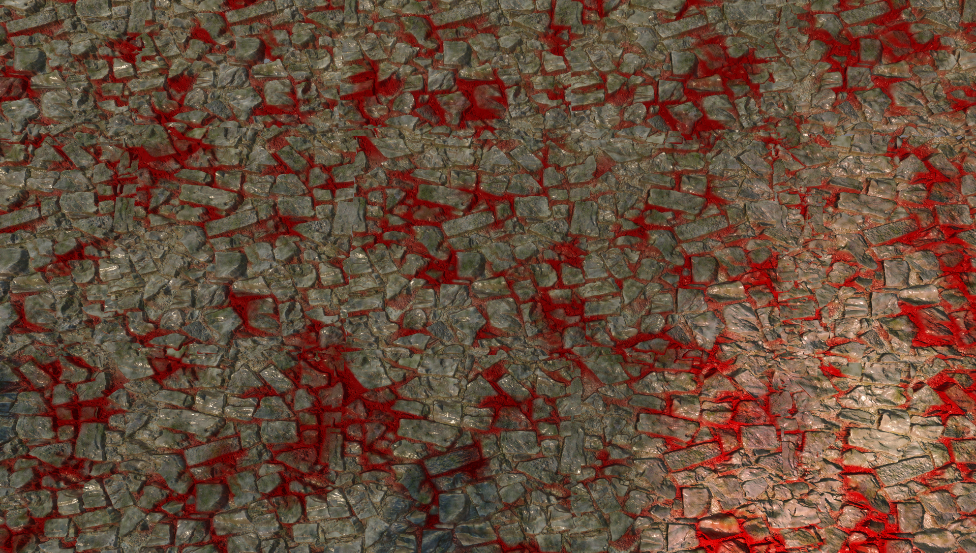
For the material shader, I wanted something roughly similar to what games actually use. In test models, it’s very common to use simple PBR textures that do a quick albedo, normal, specular lookup and output them directly. But material graphs in the real world tend to look like a bowl of spaghetti. I made this shader from two sets of textures from AmbientCg.com [2], which by the way, is highly recommended if you need free, high-quality textures under a permissive license.
For blending, I used 3 octaves of Perlin noise. I also made a third layer, which I had originally planned to be a wetness layer. But my first test was flat red, which has a nice dry powder look, so that’s what I went with. It’s blended in with an octave of Perlin noise combined with the heightmap so the red layer is biased into the cracks between the stones.
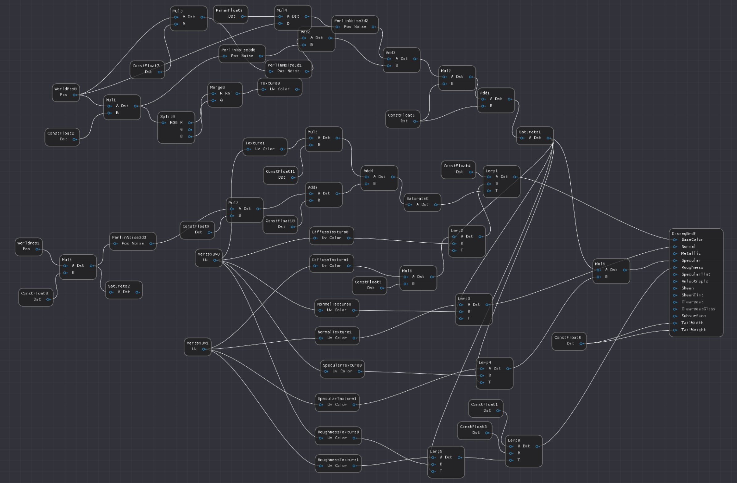
Here is a screenshot of the material graph. It’s a bit messy, as this material editor lacks most (all?) of the UI features of a proper, commercial engine. There are a lot of extra nodes because I never got around to adding constants to nodes (like adding 0.5 requires both an add node and a 0.5 constant node). But it was good enough for this test.
Low Triangle Count
For the first test, we will look at big triangles, so each mesh is just a quad made from two triangles. Here is a low view for you, so you can see how flat it is.
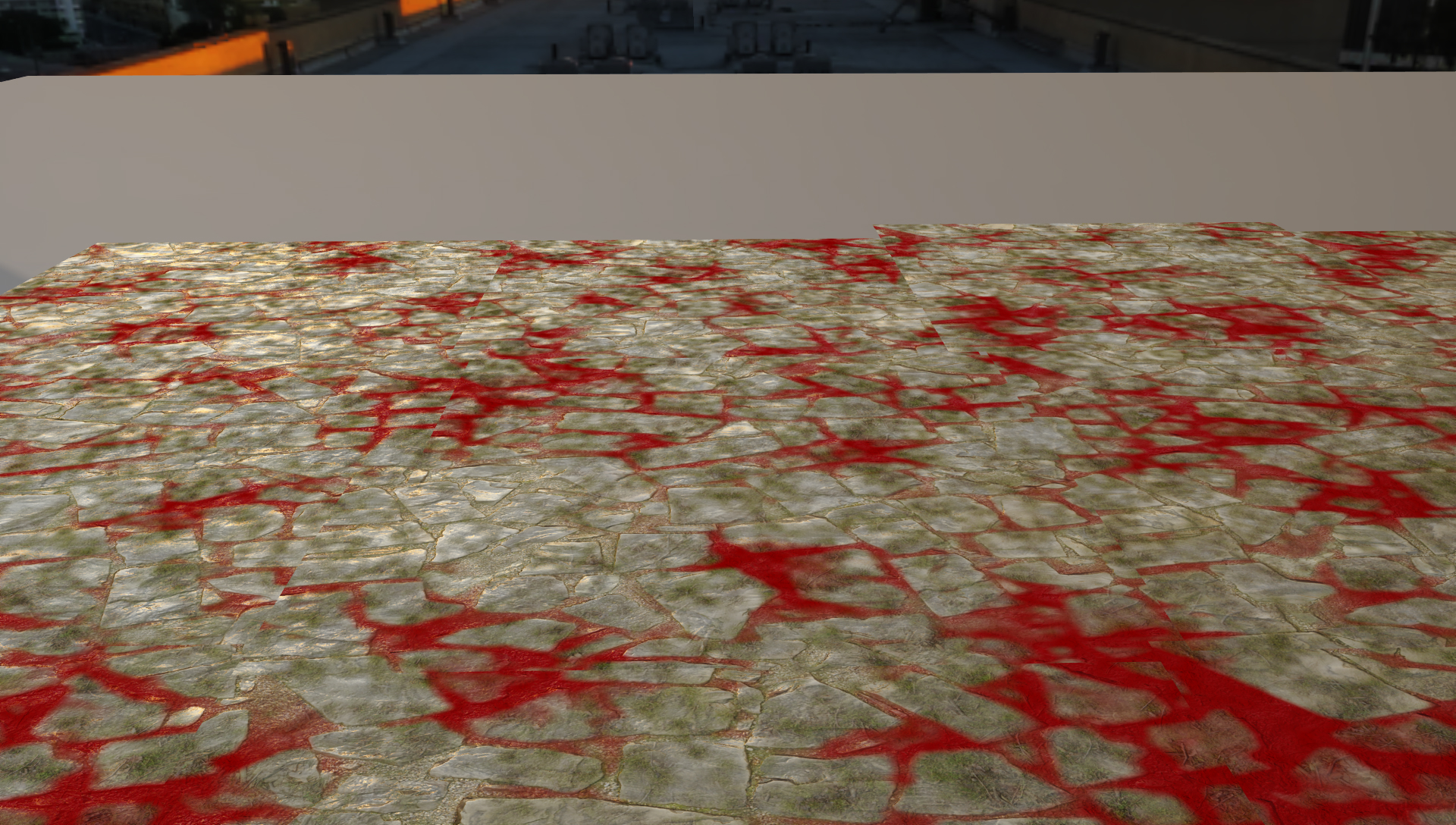
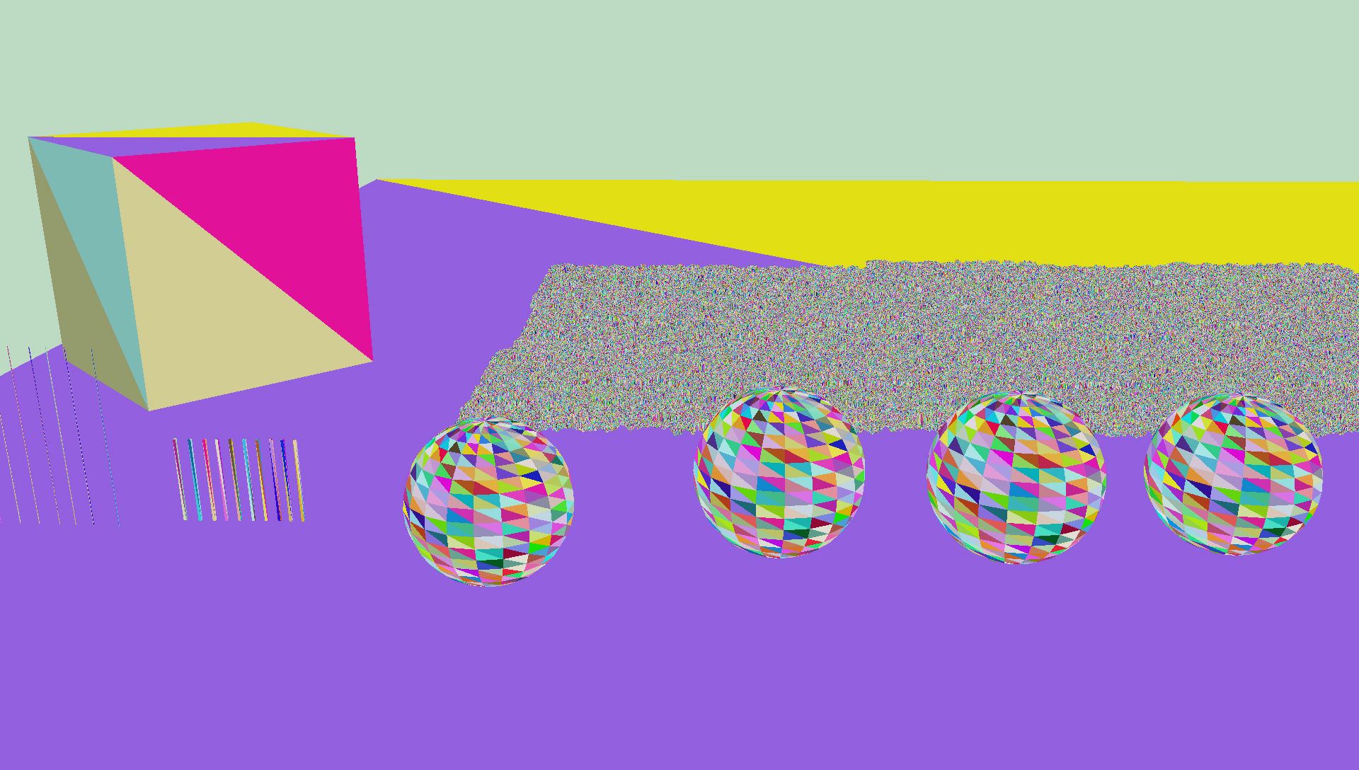
Here is the triangle ID view. As you can see, each draw call is just two triangles.

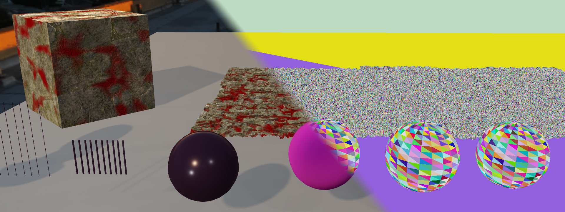
And the final image.
Let’s capture some numbers. Here is an explanation of the passes.
PrePass: For the Forward and Deferred pass, PrePass writes only depth. However, for the Visibility pass, it also writes the visibility U32 including drawCallId and triangleId.
Material: For the Deferred pass, this pass refers to the material rasterization pass. For Visibility, it refers to the time of the compute pass. And of course, for the Forward pass this is merged with the Lighting pass for one number.
Lighting: In the Deferred case, this pass is a compute shader that reads the textures and writes the lighting. Visibility does a similar operation with buffers instead of textures.
VisUtil: This category refers to the other passes in the Visibility renderer. This includes the compute shader which counts the number of pixels for each material, reorders the visibility buffer, and then reorders it back to a linear buffer when the pixels are shaded.
Other: This category refers to everything else. The main passes here are the shadow pass, TAA, motion vectors, tonemapping, GUI (which doesn’t appear in these screenshots), and miscellaneous barriers. The way I actually counted this was by taking the total GPU time and subtracting all the other categories.
The Other category is a bit tricky, as Raster/Compute overlap is one of the key design decisions in organizing your rendering passes. But for this test the goal is to determine the relative cost among different algorithms, not minimize the final render time. The cost is roughly similar for all three rendering types, so it made sense to group them separately. The choice of Forward/Deferred/Visibility has minimal effect on the cost of these items like TAA and shadows.
Low density triangle view performance.
| PrePass | Material | Lighting | VisUtil | Other | Total | |
|---|---|---|---|---|---|---|
| Forward | 0.020 | 1.61 | 0.749 | 2.379 | ||
| Deferred | 0.020 | 1.06 | 0.730 | 0.759 | 2.569 | |
| Visibility | 0.043 | 1.06 | 0.762 | 0.322 | 0.832 | 3.01 |
Well, that result is interesting. In the deferred case, the Material shader cost is 1.06ms, and the visibility shader cost is, somehow, exactly the same at 1.06ms. Additionally, the lighting shader cost is slightly higher by 0.032ms, and it has an extra 0.322ms of overhead in managing the visibility passes. Finally, the forward pass can calculate Material and Lighting slightly faster, likely because it is saving on bandwidth.
First, as a disclaimer, the 5x3 quads are nearly flat, and there is a little z-fighting, so it’s plausible that some pixels in the GBuffer pass are not getting correct early-z rejection, causing a small amount of overdraw. But the more likely explanation is that the pass is primarily bandwidth limited, so the extra ALU cost of interpolating vertices and calculating derivatives is hidden by the bandwidth cost.
But, looking at the numbers, the extra cost of fetching the vertex attributes and calculating the partial derivatives is…nothing? The Visibility lighting pass is slightly higher, and the extra management passes add up, but overall that’s a very encouraging result for the next test. Also, the VisUtil pass could likely come down a bit. The current implementation renders the Lighting using buffers instead of textures, and sorts the data later. But clearly it would be faster to store the output of the Visibility Data directly into the GBuffer as UAVs.
Medium Triangle Count
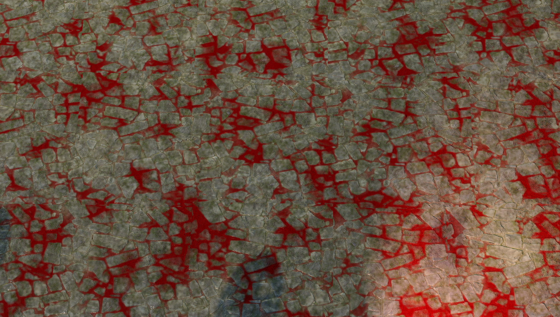
Next up, let’s try a medium-resolution view. For the high-res image, we will be at 500x500. To get pixels 10x lighter we can make them a resolution of 500/sqrt(10)=158. Thus, the meshes for this medium-resolution setup are 158x158. They have detail but are definitely on the lumpy side.
Here is the final view from our camera angle:
And of course, the view of all the triangles. When angling the camera, I was trying for about 10 pixels per triangle, but at a glance it seems closer to 8. The goal is to capture the trend, not any specific size, so it’s good enough.

Given that triangles are about 8-10 pixels, we would expect about the cost to be about 2x for any rasterized passes. What are the numbers then?
| PrePass | Material | Lighting | VisUtil | Other | Total | |
|---|---|---|---|---|---|---|
| Forward | 0.132 | 3.92 | 1.099 | 5.151 | ||
| Deferred | 0.132 | 2.95 | 0.764 | 1.122 | 4.968 | |
| Visibility | 0.158 | 1.65 | 0.818 | 0.336 | 1.188 | 4.15 |
As a disclaimer, the change in Other is not significant, as the change is driven by the shadow depth passes. The shadow pass is quite naive, simply rendering all the geometry into the cascades and point light shadow passes. Since the geometry jumps in complexity, so does the shadow pass. However, this change in cost is effectively the same for all three rendering types. Let’s examine just the relevant passes for the three different algorithms: PrePass, Material, Lighting, and VisUtil.
| PrePass + Material + Lighting + VisUtil | |
|---|---|
| Forward (M) | 4.05 |
| Deferred (M) | 3.85 |
| Visibility (M) | 2.96 |
Looking at the numbers, it’s clear that as triangles get smaller, Visibility rendering pulls ahead. And the numbers are not as close as I thought they would be. The first thing I actually noticed was the PrePass. I had expected more of a performance impact from rendering both Visibility ID and Depth (as opposed to only depth), but the cost difference is pretty low (0.033ms). The biggest jump is the Forward and Deferred Material passes, which get 2.43x and 2.78x the length respectively (compared to the previous first image). The Visibility Material pass is 1.56x the length of the original pass.
But why does the Visibility Material pass take longer than the big triangle case? After all it is the same shader running on the same number of pixels. The issue is cache coherency. Let’s look at two scenarios. On the left, we have an 8x8 block of pixels that are split between two triangles, and on the right each pixel in the 8x8 block points to a different triangle.
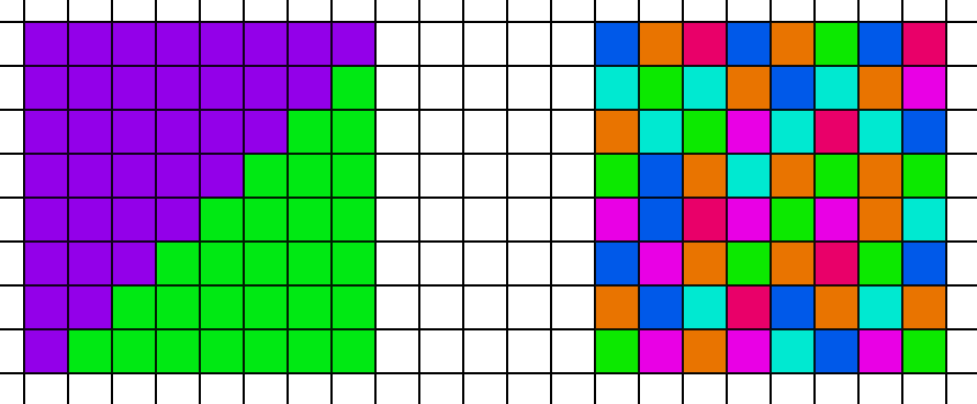
In the compute shader, all 64 threads fetch the data for the first vertex. But in the case on the left, the GPU will only need to fetch 2 unique vertex locations for the entire 8x8 block. However in the case on the right, the GPU will need to fetch from 64 unique locations in memory. In addition to worse coherency, it will also have more raw bandwidth to fetch, as the total number of bytes it needs to fetch from memory is higher. So while these extra fetches had a trivial cost in the first test case with large triangles, they have a relevant cost in this scene. However, that cost is much less than the penalty that the Deferred path pays due to poor quad utilization. Thus, the Visibility approach is faster overall.
High Triangle Count
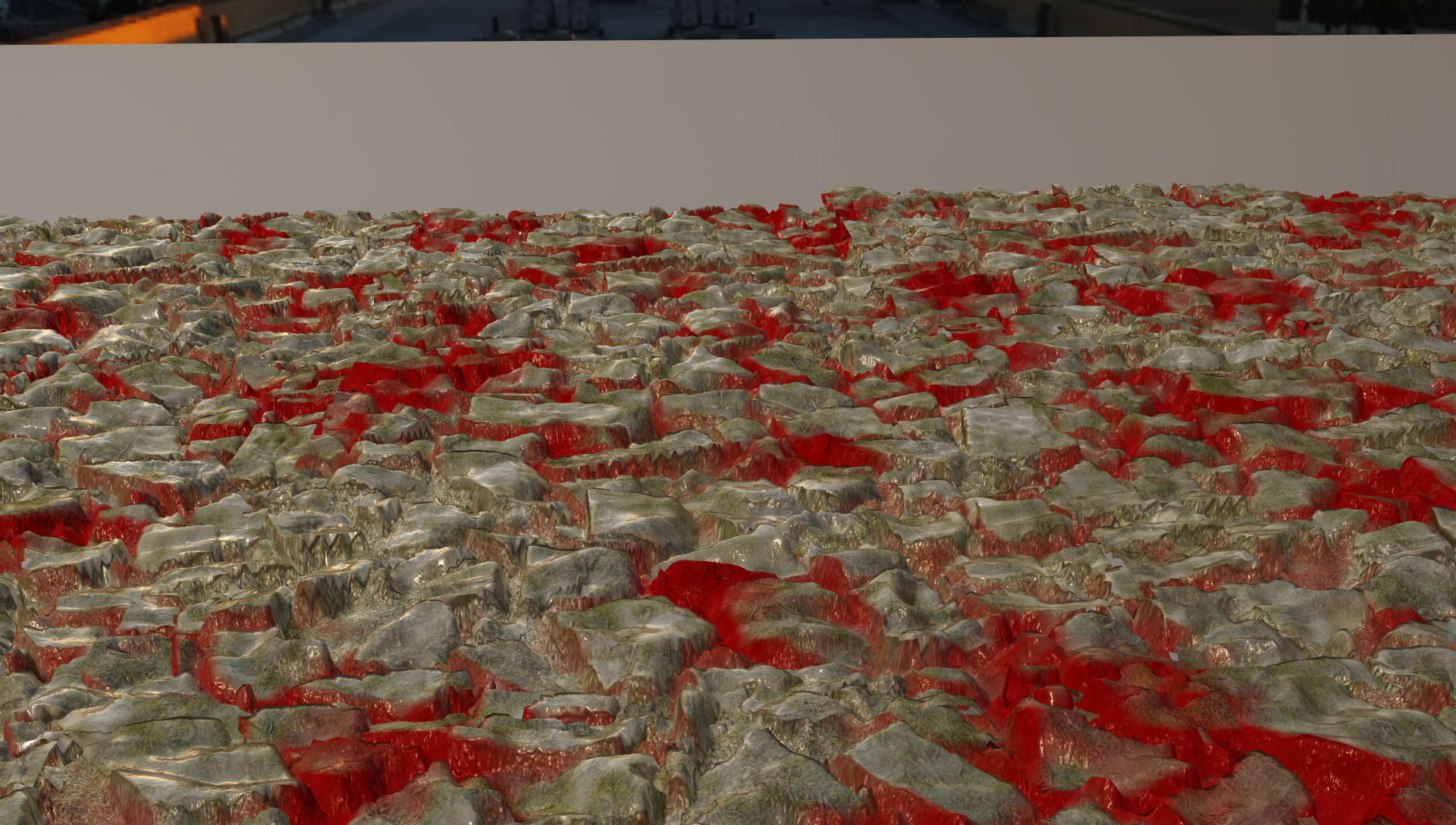
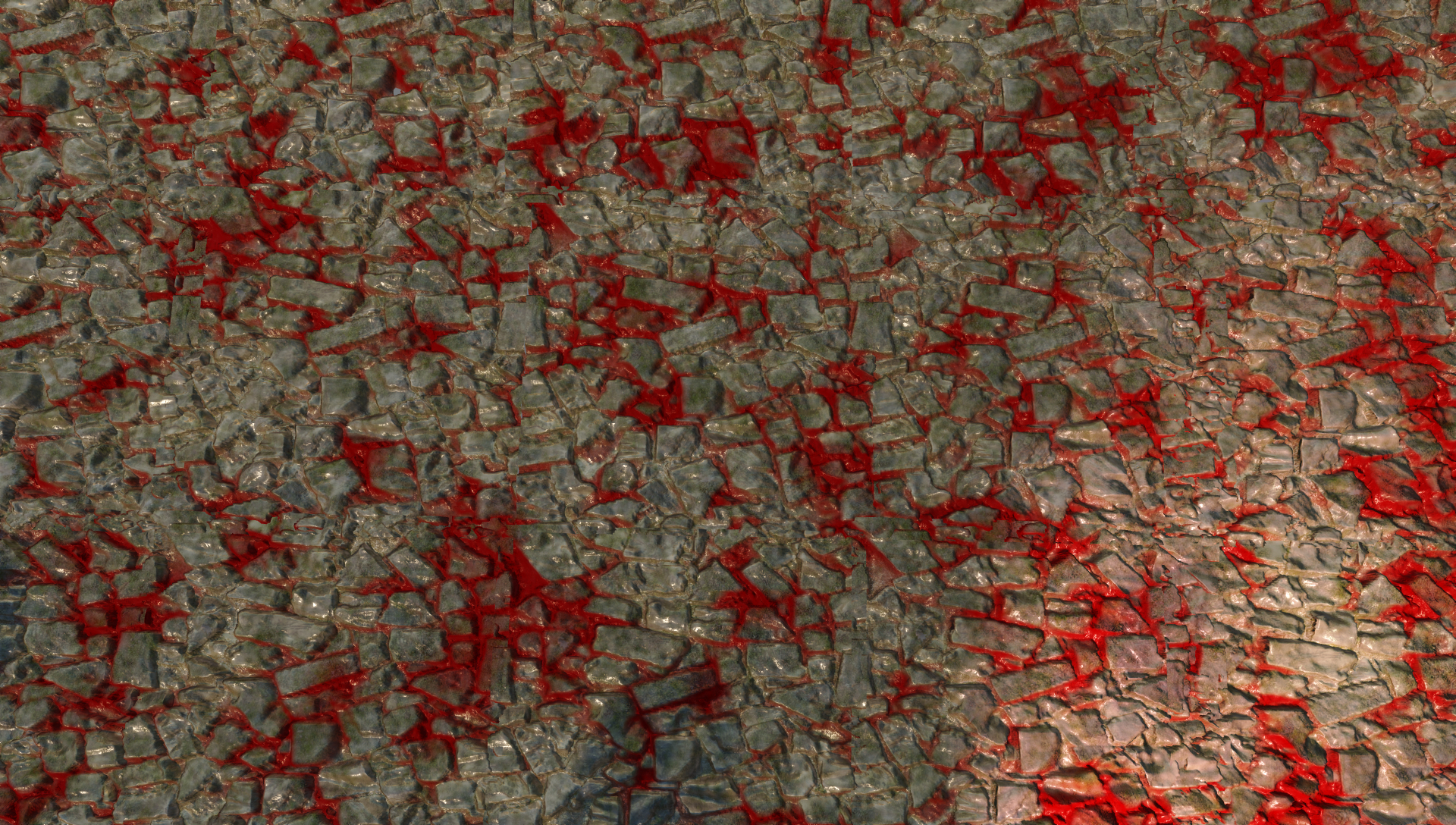
Finally, let’s do a third screenshot at a high triangle count. Each of the models is 500x500, and we are well into 1 pixel per triangle. Here is a closup of the rocks.
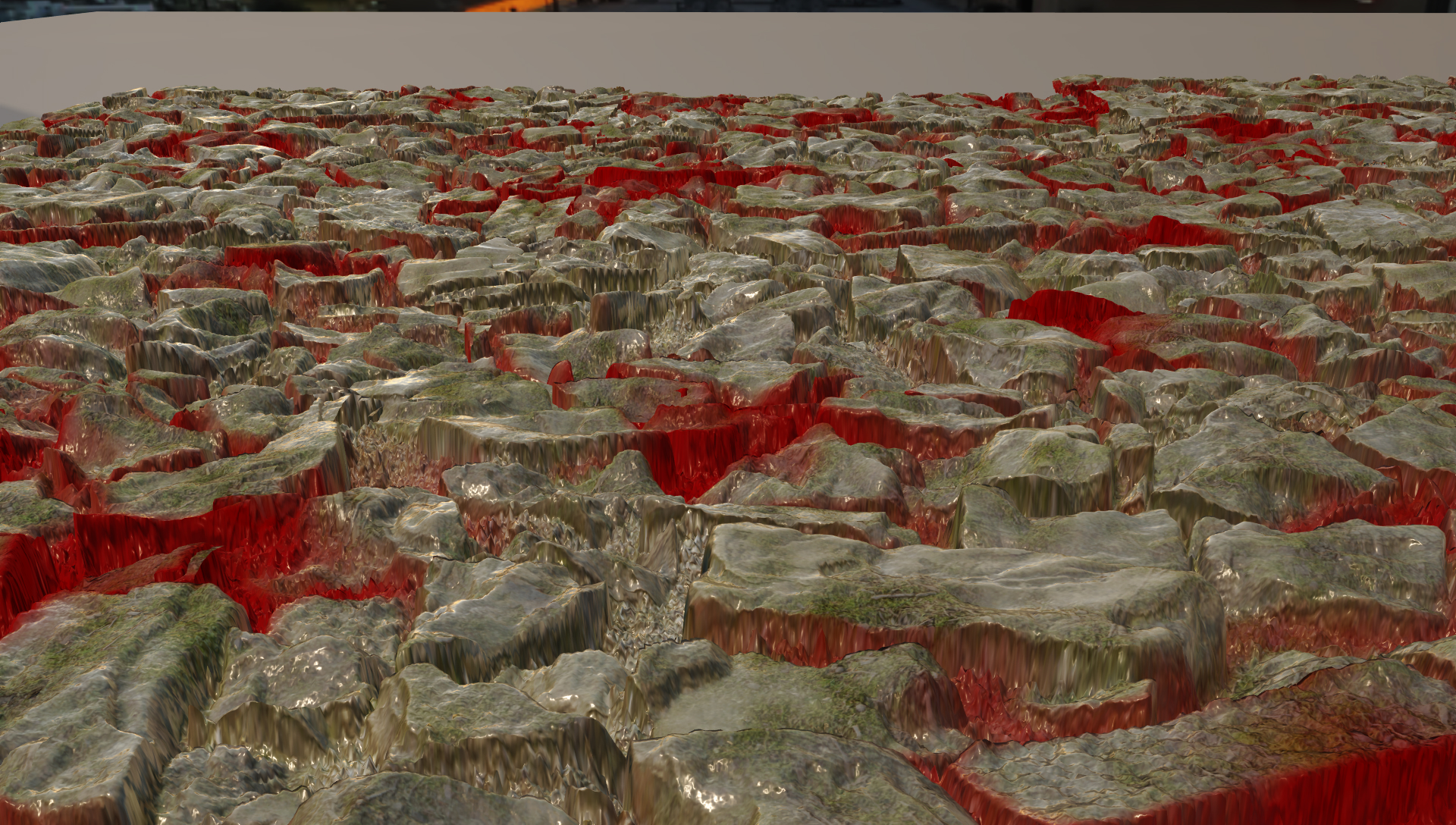
The final image:
And the triangle ids:

So what do the numbers look like?
| PrePass | Material | Lighting | VisUtil | Other | Total | |
|---|---|---|---|---|---|---|
| Forward | 1.00 | 9.27 | 4.726 | 14.996 | ||
| Deferred | 1.00 | 4.64 | 0.792 | 4.729 | 11.161 | |
| Visibility | 1.15 | 2.01 | 0.836 | 0.341 | 4.516 | 8.853 |
Starting the timeline, the PrePass cost goes up but stays reasonable, and the cost of writing the Visibility U32 only adds 15%. The Other pass also goes up significantly but that is primarily driven by the shadow depth pass. The visibility pass is 0.21ms less in the Other category, which is a little strange. Looking at the PIX run, the shadow depth pass does have some overlap with the PrePass, so it’s possible that the extra 0.15ms cost of the PrePass is hiding 0.15ms of the shadow pass and the other 0.06ms is hidden by other overlap with VisUtil.
But the major difference is the Material and Lighting costs. The numbers pretty much speak for themselves. The Forward cost scales by 5.76x compared to the first frame, and the Deferred Material cost increases by scales to 4.38x of the first frame. However, the Visiblity Material cost scales by 1.90x of the first frame.
Once again, let’s isolate the passes relevant to the differences between the rendering algorithms.
| PrePass + Material + Lighting + VisUtil | |
|---|---|
| Forward (H) | 10.27 |
| Deferred (H) | 6.43 |
| Visibility (H) | 4.34 |
The numbers are clear. In this test case, once triangle density reduces to a single pixel, the better quad utilization of Visibility rendering greatly outweighs the additional cost of interpolating vertex attributes and analytically calculating partial derivatives.
Conclusions:
Getting back to the original questions:
Can we efficiently calculate analytic partial derivatives with material graphs?
In this test case, the answer is “yes”. But in the general case, the better answer is “maybe”. The extra calculations needed to generate partial derivatives are trivial in the simple cases of UV scales and offsets. I did some other cursory tests (without doing a full set of PIX runs) and at a glance there are no critical use cases that would cause enough of a performance penalty to fundamentally change the numbers.
The most common case would be a texture output that becomes a UV for another texture. If we have a standard material with 4 texture reads, and then we add a UV offset texture read, the Forward/Deferred Material pass would add 1 texture read whereas the Visibility Material pass would add 3. But the difference between 5 and 7 texture samples will not cause a performance cliff strong enough to drastically change the numbers. And I would expect those two extra samples to have minimal cost since they will be very cache-coherent with the first one.
A more problematic case is Parallax Occlusion Mapping. In theory we would need 3 texture reads instead of 1 for each step. But would the derivatives actually change that much from each step? Would it be acceptable to use the same derivatives/mip-map level for all of them? At a glance it seems reasonable, but I haven’t verified.
And of course, we have the really bad cases. A refraction eye shader would need to pass along the partial derivative of the view vector as it refracts with the cornea geometry normal. I could imagine that shader being 3x slower than the finite differences version, since we need to account for the derivatives of the view vector w.r.t. x and y and also the partial derivatives of the cornea height and normal w.r.t. x and y. But I can also think of approximations that would reduce the cost. For example, I suspect we could assume the curvature of the cornea is too small to be relevant and we could make that derivative zero in the calculations.
Finally, standard derivatives using finite differences are not perfect either. We have problematic cases like branches and discard which are elegantly solved by switching to analytic derivatives. This is especially true when using helper lanes that go off the edge of the triangle.
So yes, it works in this case. But for the general problem of partial derivatives in AAA games, my answer is “maybe, with a lean towards yes”. My conclusion is that analytic partial derivatives are likely viable, but the approach would need more testing to be sure for the more complicated use cases.
For very high triangle counts (1 pixel per triangle), is the Visibility approach faster?
For very high triangle counts, where each pixel is run 4 times, Visibility rendering is a clear winner. The Deferred cost is 6.43ms compared to 4.34ms for Visibility. A 32.5% reduction in overall GPU cost for the relevant passes is non-trivial.
What about more typical triangle sizes (5-10 pixels per triangle)? Is the Visibility approach faster there too?
For medium counts, in these tests, yes, the visibility approach is faster as well. The margin is closer though, at 3.85ms vs 2.96ms. Still, a 23.1% reduction is non-trivial. Additionally, I would expect the Visibility approach to be less spikey in the bad view angles with lots of geometry and overdraw, but that’s conjecture.
Other Considerations:
Given that Visibility rendering scales better than Deferred for high triangle counts, and triangle counts are going up every year, should every game engine drop everything and switch? Of course not. There are several other factors in any major architectural rendering decision.
Code Complexity:
Probably the best argument against Visibility rendering is the complexity involved. Visibility rendering requires engineering time to manage vertex buffers and partial derivatives. Engineering time is not infinite.
Memory:
In order to use Visibility rendering, all of your dynamic geometry needs to be in a giant buffer (or buffers) that can be accessed from a shader. If your screen is covered in blades of grass, every single one of those post-deformation vertices needs to be in a buffer somewhere. That being said, the memory is not necessarily as bad as it sounds. You can probably pack position XYZ into 16 bits each, so each vertex is 6 bytes. If you need a post-deformation tangent space you can store that in a 4 byte quaternion, for 10 bytes per pixel total. Suppose you are rendering at 1080p (2 million pixels), and you have one vertex per pixel. That puts you at 20MB of RAM, or 40MB if you need to store the previous frame too. 40MB of RAM is not trivial, but it is not ridiculous either. And if you want to include the mesh in raytracing you need the post-deformation vertices anyways.
PSO Switches:
One of the subtle advantages of Visibility rendering is fewer PSO switches during rasterization. In a Forward or Deferred rasterization pass, bubbles can form when the Pixel Shader is starved for work from the earlier stages, especially if the PSO is constantly switching. But opaque geometry can share the same Visibility pixel shader despite having a completely different material. While there are a few exceptions (backface culling, alpha testing, etc), we can group all visible geometry into only a few PSOs for the triangle ID writing pass. We can also more aggressively group PSOs in the material pass. For example, a material that renders opaque and a variation with alpha-testing can evaluate the material data in the same Visibility indirect CS dispatch, whereas they would require separate PSOs in a Deferred material pass. The Visibility pipeline should have significantly fewer bubbles, but testing that kind of workload is beyond the scope of a small toy engine.
Material Cost:
If you are rendering with giant, complex materials, then visibility is more compelling. That’s because the cost of fetching and interpolating your vertex data is hidden by the cost of material evaluation. If you are rendering with short material shaders, then the interpolation cost will be more exposed, as well as the fixed cost overhead.
Min-Spec:
These tests were performed on an NVIDIA GTX 3070, which is higher than the min-spec of any AAA game coming out in the near future. In particular, this test case has about 0.34ms of fixed cost. However, that same cost on a low-end laptop GPU from 5 years ago is going to be quite steep. Visibility scales well for future GPUs which will be even more powerful, but by the same token it scales poorly for past GPUs that will be in the min-spec for a long time.
Resolution Upscaling:
A secondary consideration is the role of upscaling algorithms, such as NVIDIA’s DLSS [10], AMD’s Super Resolution [1], and Unreal’s Temporal Super Resolution [6]. Opinions differ of course, but if I could choose between a 4k native resolution with cut-down shading versus a really good 1080p image with high quality shading upscaled to 4k, I’d take the upscaled 1080p. But suppose that you are targeting a 4k image with 10 pixels per triangle, and then you decide to switch to 1080p. Well, suddenly your 10-pixel triangles become 2.5-pixel triangles. In other words, if we push the triangle count from the PS4/XB1 but keep our resolutions targeting 1080p framebuffers, then we are going to have a whole lot of very small triangles on PS5/XSX.
Quad Utilization Matters:
Really, the big conclusion here is that Quad Utilization matters. It is effectively the same cost as overdraw! We all know that 1 pixel triangles are bad, but 10 pixel triangles are not ideal either. 4x is worse than 2x, but 2x is also worse than 1x. Quad utilization is not a distant problem for the future. It is a real issue today in the workloads that games are actually shipping with. But if we do address quad utilization, we actually have a lot of room to optimize our renderers and use those GPU cycles for interesting effects instead of helper lanes.
REFERENCES:
[1] AMD FidelityFX, Super Resolution. AMD Inc. (https://www.amd.com/en/technologies/radeon-software-fidelityfx-super-resolution)
[2] AbientCG, (https://www.ambientcg.com)
[3] The Visibility Buffer: A Cache-Friendly Approach to Deferred Shading. Christopher Burns and Warren Hunt. (http://jcgt.org/published/0002/02/04/)
[4] ConfettiFX/The-Forge. ConfettiFX. (https://github.com/ConfettiFX/The-Forge)
[5] 4K Rendering Breakthrough: The Filtered and Culled Visibility Buffer. Wolfgang Engel. (https://www.gdcvault.com/play/1023792/4K-Rendering-Breakthrough-The-Filtered)
[6] Unreal Engine 5 Early Access Release Notes. Epic Games, Inc. (https://docs.unrealengine.com/5.0/en-US/ReleaseNotes/)
[7] Nanite, Inside Unreal. Brian Karis, Chance Ivey, Galen Davis, and Victor Brodin. (https://www.youtube.com/watch?v=TMorJX3Nj6U)
[8] Sony Pictures Imageworks Arnold. Christopher Kulla, Alejandro Conty, Clifford Stein, and Larry Gritz. (https://dl.acm.org/doi/10.1145/3180495)
[9] HLSL Shader Model 6.0, Microsoft Inc. (https://docs.microsoft.com/en-us/windows/win32/direct3dhlsl/hlsl-shader-model-6-0-features-for-direct3d-12)
[10] NVIDIA DLSS. NVIDIA Inc. (https://www.nvidia.com/en-us/geforce/technologies/dlss/)
[11] Automatic Differentiation, C++ Template and Photogrammetry. Dan Piponi. (http://citeseerx.ist.psu.edu/viewdoc/download?doi=10.1.1.89.7749&rep=rep1&type=pdf)
[12] Deferred Attribute Interpolation for Memory-Efficient Deferred Shading. Cristoph Schied and Carsten Dachsbacher. (http://cg.ivd.kit.edu/publications/2015/dais/DAIS.pdf)