Can we use multisampling effectively for upsampling? This has been a question in the back of my mind for give or take 10+ years.
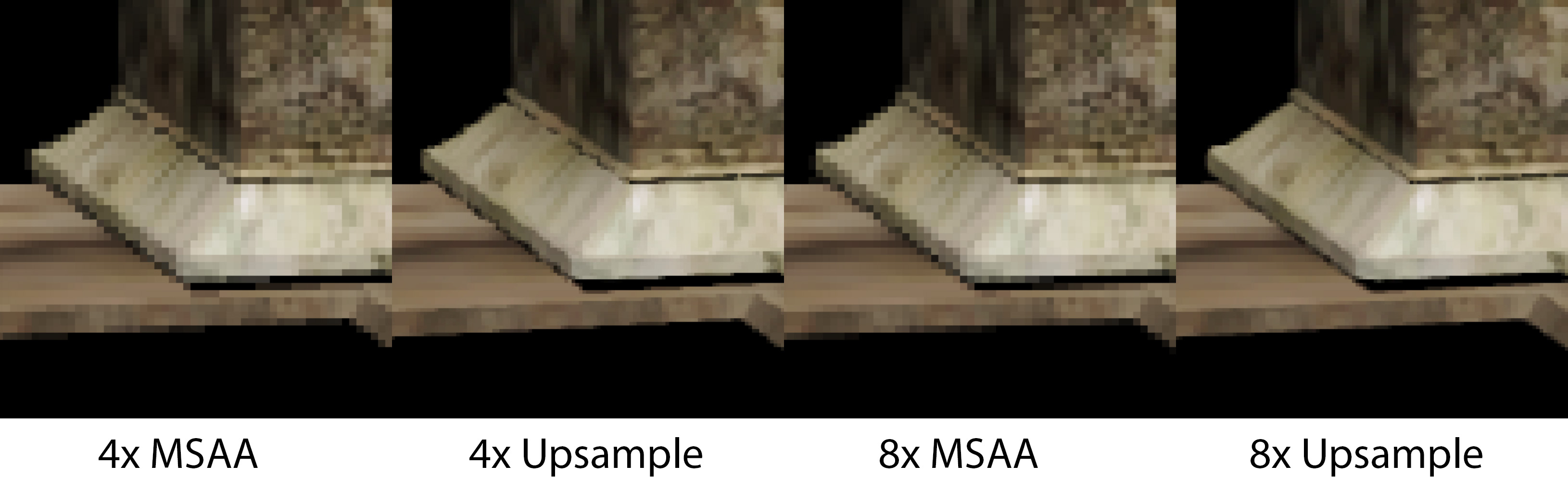
In the image at the top, the left images shows a standard 4x MSAA scene resolved to 1x by averaging the 4 sample points. The second image uses the exact same source MSAA render target, but upsamples to 4x area scaling (2x in each dimension). Similarly, the third image shows an 8x scene resolved to 1x by averaging the samples, while the fourth image is upsampling to 4x area as well. It is a pretty simple idea, and it seems like something that someone has probably tried, but I can not find any references to it so here we are.
I specifically remember thinking about this problem as I was reading Matt Pettineo’s article Experimenting with Reconstruction Filters for MSAA Resolve (while Kenny Loggins played in the background) [9]. It always seemed like there must be a good way to use the jittered sample information in a useful way to upsample the image. I have looked around for references to doing this, but I have not found many hits on the web (of course, please ping me if there are important references that I missed).
Then I saw this post from Timothy Lottes and it sent me down a deep rabbit hole.
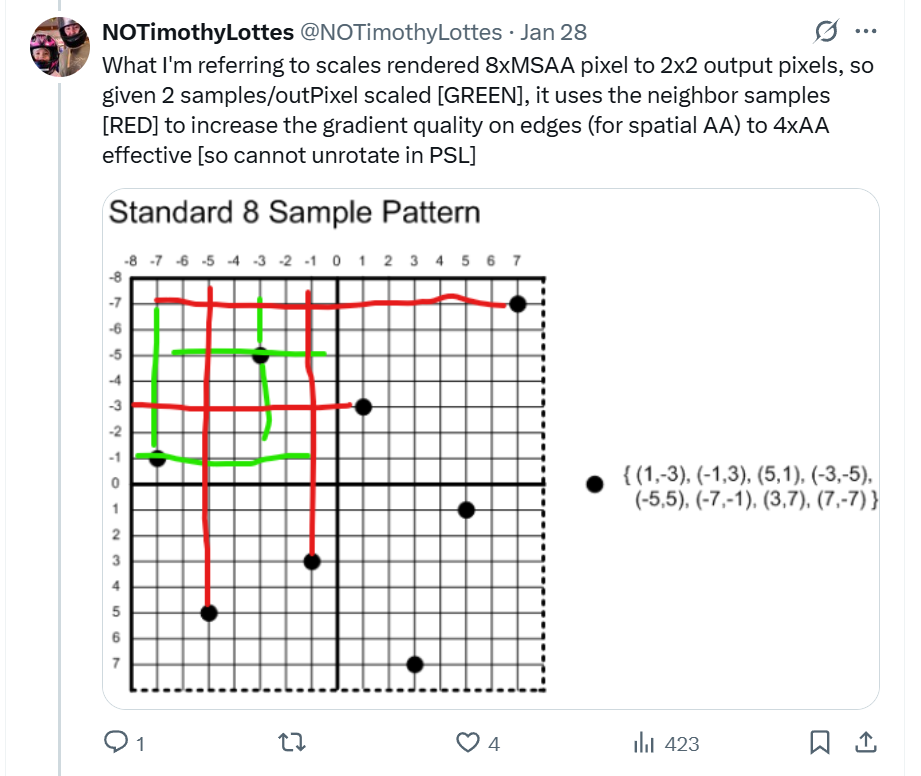
When I saw this post, I nearly jumped out of my seat. I ran into the exact same problem several years ago in my own upsampling adventures and I never figured out a good solution. But this is such a simple, elegant solution to the problem. And it got me thinking about how to use a trick like that for general purpose multisample upsampling.
In the most typical case, we would render to 1080p with 2x/4x/8x MSAA, and we want to upsample the result to 4k (3840x2160). We do not have any other buffers or temporal information. And we want to do it in one pass to keep the bandwidth down. Can we use the multisampled data in a meaningful way?
2x MSAA Upsampling to 4x Area
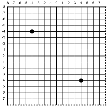
Let us start with the 2x case. The sample pattern for 2x is very simple [7]. If you split the pixel into 4 quads, you get one sample in the upper left and one sample in the lower right.
Here is an example image showing a comparison between a naive resolve which averages the colors together, versus the two diagonal samples that make up that pixel with black pixels in the missing areas.
The left shows the naive resolve. The right shows the two original samples.
Thus the question becomes: How should we fill those black pixels? We can start with a synthetic example where three of the neighbors are red and one is blue.
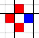
The obvious solution would be the average of all four pixels, but that actually causes problems, especially on edges. On edges, it causes a “zipper” pattern, where the pixels inside and outside the “teeth” of the edge alternate colors. Fortunately, there is a better algorithm called “smallest absolute difference” which means you pick the edge with a smaller gradient.
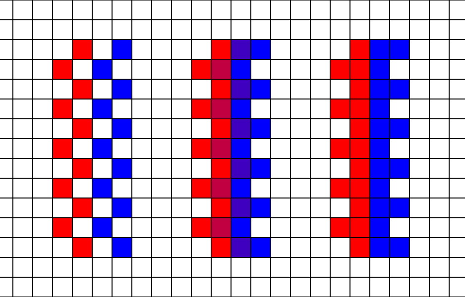
The left shows the original pixel with empty pixels in white. The middle shows the zipper pattern from linear interpolation. The right side fills the missing pixels using the smallest absolute difference.
There are other more complex methods, but smallest absolute difference is cheap and effective. At a minimum, the smallest absolute difference result looks much cleaner than the average of all 4 neighbors.
A linear resolve from averaging all four samples (left) vs using the edge from smallest absolute difference (right).
Also, note that this algorithm is very well known. The original use that I could find is from debayering with VNG [18] in DCRAW [8]. But I have also seen it with checkerboard rendering [17][3][1], as well as a component of SMAA 2x [10]. The example code is below. How you calculate luminance is up to you, but I generally prefer the 25% red, 50% green, 25% blue approach.
float3 CalcDiamondAbsDiff(float3 left, float3 right, float3 up, float3 down)
{
	float lumL = CalcLuminance(left);
	float lumR = CalcLuminance(right);
	float lumU = CalcLuminance(up);
	float lumD = CalcLuminance(down);

	float diffH = abs(lumL - lumR);
	float diffV = abs(lumU - lumD);

	float3 avgH = (left + right) * .5f;
	float3 avgV = (up + down) * .5f;

	float3 ret = (diffH < diffV) ? avgH : avgV;

	return ret;
}
As an aside, there are other options instead of using the smallest absolute difference. For example, Rainbow Six Siege used linear interpolation with an explicit “unteething” filter [17].
4x MSAA Upsampling to 4x Area
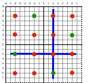
Next up, how about 4x? The jittered grid MSAA pattern looks like so.
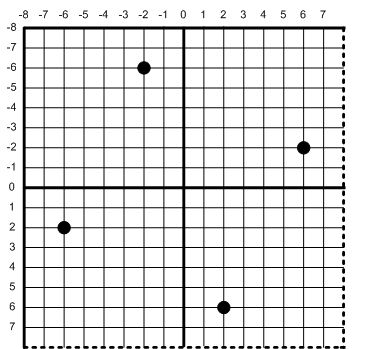
We have these points which have a known color (in green), and these red points that are unknown (in red). Each upsampled pixel (at 4x area scaling) has one green and three reds. Each red point can be estimated from the 4 neighboring green points using smallest absolute difference. Then we can add up all points in the upsampled pixel, and if we can calculate a good estimate of all three, then each of those upsampled pixels would theoretically have AA quality roughly equal to 2x MSAA.
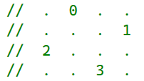
For simplicity, I prefer to think about one of the original MSAA pixels as a 4x4 grid with 4 samples. In a single pixel, the 4 locations of the samples are listed below.
If we want to calculate all 16 points (4 known, 12 unknown), we need to look at at the neighbors as well.
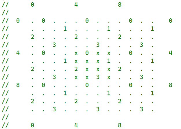
We want to calculate the color of the xs in the grid. The first step is to fetch the known values in the grid. This is obviously not the fastest way to do it, but it keeps things simple for now.
int2 srcXy = dispatchThreadId.xy;

int halfX0 = max(0,srcXy.x-1);
int halfX1 = srcXy.x;
int halfX2 = min(sizeX-1,srcXy.x+1);

int halfY0 = max(0,srcXy.y-1);
int halfY1 = srcXy.y;
int halfY2 = min(sizeY-1,srcXy.y+1);

float3 color__0__5 = texData.Load(int2(halfX1,halfY0),0).xyz;
float3 color__1__7 = texData.Load(int2(halfX1,halfY0),1).xyz;
float3 color__2__4 = texData.Load(int2(halfX1,halfY0),2).xyz;
float3 color__3__6 = texData.Load(int2(halfX1,halfY0),3).xyz;

float3 color__4__1 = texData.Load(int2(halfX0,halfY1),0).xyz;
float3 color__5__3 = texData.Load(int2(halfX0,halfY1),1).xyz;
float3 color__6__0 = texData.Load(int2(halfX0,halfY1),2).xyz;
float3 color__7__2 = texData.Load(int2(halfX0,halfY1),3).xyz;
float3 color__4__5 = texData.Load(int2(halfX1,halfY1),0).xyz;
float3 color__5__7 = texData.Load(int2(halfX1,halfY1),1).xyz;
float3 color__6__4 = texData.Load(int2(halfX1,halfY1),2).xyz;
float3 color__7__6 = texData.Load(int2(halfX1,halfY1),3).xyz;
float3 color__4__9 = texData.Load(int2(halfX2,halfY1),0).xyz;
float3 color__5_11 = texData.Load(int2(halfX2,halfY1),1).xyz;
float3 color__6__8 = texData.Load(int2(halfX2,halfY1),2).xyz;
float3 color__7_10 = texData.Load(int2(halfX2,halfY1),3).xyz;

float3 color__8__5 = texData.Load(int2(halfX1,halfY2),0).xyz;
float3 color__9__7 = texData.Load(int2(halfX1,halfY2),1).xyz;
float3 color_10__4 = texData.Load(int2(halfX1,halfY2),2).xyz;
float3 color_11__6 = texData.Load(int2(halfX1,halfY2),3).xyz;
Then we need to calculate all 16 grid points.
float3 grid__4__4 = CalcDiamondAbsDiff(color__4__1,color__4__5,color__2__4,color__6__4);
float3 grid__4__5 = color__4__5;
float3 grid__4__6 = CalcDiamondAbsDiff(color__4__5,color__4__9,color__3__6,color__7__6);
float3 grid__4__7 = CalcDiamondAbsDiff(color__4__5,color__4__9,color__1__7,color__5__7);

float3 grid__5__4 = CalcDiamondAbsDiff(color__5__3,color__5__7,color__2__4,color__6__4);
float3 grid__5__5 = CalcDiamondAbsDiff(color__5__3,color__5__7,color__4__5,color__8__5);
float3 grid__5__6 = CalcDiamondAbsDiff(color__5__3,color__5__7,color__3__6,color__7__6);
float3 grid__5__7 = color__5__7;

float3 grid__6__4 = color__6__4;
float3 grid__6__5 = CalcDiamondAbsDiff(color__6__4,color__6__8,color__4__5,color__8__5);
float3 grid__6__6 = CalcDiamondAbsDiff(color__6__4,color__6__8,color__3__6,color__7__6);
float3 grid__6__7 = CalcDiamondAbsDiff(color__6__4,color__6__8,color__5__7,color__9__7);

float3 grid__7__4 = CalcDiamondAbsDiff(color__7__2,color__7__6,color__6__4,color_10__4);
float3 grid__7__5 = CalcDiamondAbsDiff(color__7__2,color__7__6,color__4__5,color__8__5);
float3 grid__7__6 = color__7__6;
float3 grid__7__7 = CalcDiamondAbsDiff(color__7__6,color__7_10,color__5__7,color__9__7);
Then merge the grid points into the 4x area pixels….
float3 dst00 = 0.25f*(grid__4__4 + grid__4__5 + grid__5__4 + grid__5__5);
float3 dst01 = 0.25f*(grid__4__6 + grid__4__7 + grid__5__6 + grid__5__7);
float3 dst10 = 0.25f*(grid__6__4 + grid__7__5 + grid__6__4 + grid__7__5);
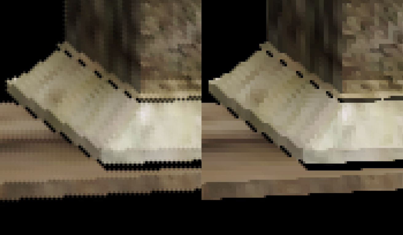
float3 dst11 = 0.25f*(grid__6__6 + grid__7__7 + grid__6__6 + grid__7__7);And finally we can just write the 4 pixels and we are done. So how does it look? Honestly, not too shabby.
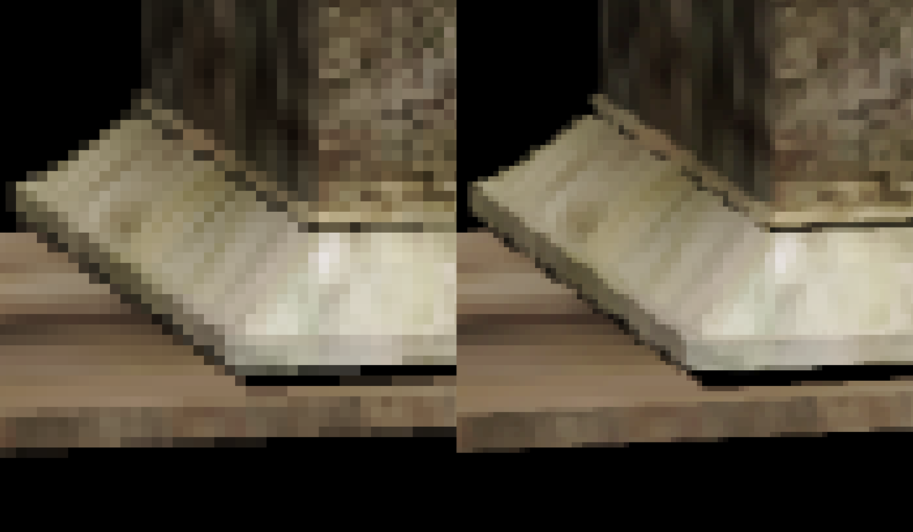
A naive resolve of the 4x MSAA image (left) and the upsampled resolve (right).
8x MSAA Upsampling to 4x Area
And finally we are back to the original problem: 8x. At 4x area upsampling, we could potentially just pick the two samples in that region. That is actually what I did in a previous post, and I had the expected “saw-tooth” artifacts as a result. But we can do better and reconstruct the edges.
The source pixel has 8 MSAA sample points. Then when we split it into 4 output pixels, each output pixel has 2 known and 14 unknown points. The pattern looks like this:
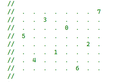
And then the entire tile grid with 1 ring of neighbor source pixels:
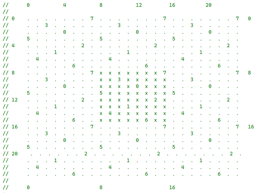
Now we have to manually write out all the intersections. I considered writing a script to do this, but it was easier just to do it by hand.
First up is the source points.
float3 color__0_15 = texData.Load(int2(halfX1,halfY0),7).xyz;
float3 color__1_10 = texData.Load(int2(halfX1,halfY0),3).xyz;
float3 color__2_12 = texData.Load(int2(halfX1,halfY0),0).xyz;
float3 color__3__8 = texData.Load(int2(halfX1,halfY0),5).xyz;
float3 color__4_14 = texData.Load(int2(halfX1,halfY0),2).xyz;
float3 color__5_11 = texData.Load(int2(halfX1,halfY0),1).xyz;
float3 color__6__9 = texData.Load(int2(halfX1,halfY0),4).xyz;
float3 color__7_13 = texData.Load(int2(halfX1,halfY0),6).xyz;

float3 color__8__7 = texData.Load(int2(halfX0,halfY1),7).xyz;
float3 color__9__2 = texData.Load(int2(halfX0,halfY1),3).xyz;
float3 color_10__4 = texData.Load(int2(halfX0,halfY1),0).xyz;
float3 color_11__0 = texData.Load(int2(halfX0,halfY1),5).xyz;
float3 color_12__6 = texData.Load(int2(halfX0,halfY1),2).xyz;
float3 color_13__3 = texData.Load(int2(halfX0,halfY1),1).xyz;
float3 color_14__1 = texData.Load(int2(halfX0,halfY1),4).xyz;
float3 color_15__5 = texData.Load(int2(halfX0,halfY1),6).xyz;
float3 color__8_15 = texData.Load(int2(halfX1,halfY1),7).xyz;
float3 color__9_10 = texData.Load(int2(halfX1,halfY1),3).xyz;
float3 color_10_12 = texData.Load(int2(halfX1,halfY1),0).xyz;
float3 color_11__8 = texData.Load(int2(halfX1,halfY1),5).xyz;
float3 color_12_14 = texData.Load(int2(halfX1,halfY1),2).xyz;
float3 color_13_11 = texData.Load(int2(halfX1,halfY1),1).xyz;
float3 color_14__9 = texData.Load(int2(halfX1,halfY1),4).xyz;
float3 color_15_13 = texData.Load(int2(halfX1,halfY1),6).xyz;
float3 color__8_23 = texData.Load(int2(halfX2,halfY1),7).xyz;
float3 color__9_18 = texData.Load(int2(halfX2,halfY1),3).xyz;
float3 color_10_20 = texData.Load(int2(halfX2,halfY1),0).xyz;
float3 color_11_16 = texData.Load(int2(halfX2,halfY1),5).xyz;
float3 color_12_22 = texData.Load(int2(halfX2,halfY1),2).xyz;
float3 color_13_19 = texData.Load(int2(halfX2,halfY1),1).xyz;
float3 color_14_17 = texData.Load(int2(halfX2,halfY1),4).xyz;
float3 color_15_21 = texData.Load(int2(halfX2,halfY1),6).xyz;

float3 color_16_15 = texData.Load(int2(halfX1,halfY2),7).xyz;
float3 color_17_10 = texData.Load(int2(halfX1,halfY2),3).xyz;
float3 color_18_12 = texData.Load(int2(halfX1,halfY2),0).xyz;
float3 color_19__8 = texData.Load(int2(halfX1,halfY2),5).xyz;
float3 color_20_14 = texData.Load(int2(halfX1,halfY2),2).xyz;
float3 color_21_11 = texData.Load(int2(halfX1,halfY2),1).xyz;
float3 color_22__9 = texData.Load(int2(halfX1,halfY2),4).xyz;
float3 color_23_13 = texData.Load(int2(halfX1,halfY2),6).xyz;
And then the crosses.
float3 grid__8__8 = CalcDiamondAbsDiff(color__8__7,color__8_15,color__3__8,color_11__8);
float3 grid__8__9 = CalcDiamondAbsDiff(color__8__7,color__8_15,color__6__9,color_14__9);
float3 grid__8_10 = CalcDiamondAbsDiff(color__8__7,color__8_15,color__1_10,color__9_10);
float3 grid__8_11 = CalcDiamondAbsDiff(color__8__7,color__8_15,color__5_11,color_13_11);
float3 grid__8_12 = CalcDiamondAbsDiff(color__8__7,color__8_15,color__2_12,color_10_12);
float3 grid__8_13 = CalcDiamondAbsDiff(color__8__7,color__8_15,color__7_13,color_15_13);
float3 grid__8_14 = CalcDiamondAbsDiff(color__8__7,color__8_15,color__4_14,color_12_14);
float3 grid__8_15 = CalcDiamondAbsDiff(color__8_15,color__8_15,color__8_15,color__8_15);

// ...

float3 grid_15__8 = CalcDiamondAbsDiff(color_15__5,color_15_13,color_11__8,color_19__8);
float3 grid_15__9 = CalcDiamondAbsDiff(color_15__5,color_15_13,color_14__9,color_22__9);
float3 grid_15_10 = CalcDiamondAbsDiff(color_15__5,color_15_13,color__9_10,color_17_10);
float3 grid_15_11 = CalcDiamondAbsDiff(color_15__5,color_15_13,color_13_11,color_21_11);
float3 grid_15_12 = CalcDiamondAbsDiff(color_15__5,color_15_13,color_10_12,color_18_12);
float3 grid_15_13 = CalcDiamondAbsDiff(color_15_13,color_15_13,color_15_13,color_15_13);
float3 grid_15_14 = CalcDiamondAbsDiff(color_15_13,color_15_21,color_12_14,color_20_14);
float3 grid_15_15 = CalcDiamondAbsDiff(color_15_13,color_15_21,color__8_15,color_16_15);
And then summing up each of our 4 output pixels.
float3 dst00 = (grid__8__8 + grid__8__9 + grid__8_10 + grid__8_11 +
                grid__9__8 + grid__9__9 + grid__9_10 + grid__9_11 +
                grid_10__8 + grid_10__9 + grid_10_10 + grid_10_11 +
                grid_11__8 + grid_11__9 + grid_11_10 + grid_11_11) * (1.0f/16.0f);

float3 dst01 = (grid__8_12 + grid__8_13 + grid__8_14 + grid__8_15 +
                grid__9_12 + grid__9_13 + grid__9_14 + grid__9_15 +
                grid_10_12 + grid_10_13 + grid_10_14 + grid_10_15 +
                grid_11_12 + grid_11_13 + grid_11_14 + grid_11_15) * (1.0f/16.0f);

float3 dst10 = (grid_12__8 + grid_12__9 + grid_12_10 + grid_12_11 +
                grid_13__8 + grid_13__9 + grid_13_10 + grid_13_11 +
                grid_14__8 + grid_14__9 + grid_14_10 + grid_14_11 +
                grid_15__8 + grid_15__9 + grid_15_10 + grid_15_11) * (1.0f/16.0f);

float3 dst11 = (grid_12_12 + grid_12_13 + grid_12_14 + grid_12_15 +
                grid_13_12 + grid_13_13 + grid_13_14 + grid_13_15 +
                grid_14_12 + grid_14_13 + grid_14_14 + grid_14_15 +
                grid_15_12 + grid_15_13 + grid_15_14 + grid_15_15) * (1.0f/16.0f);
And that ends up working pretty well.
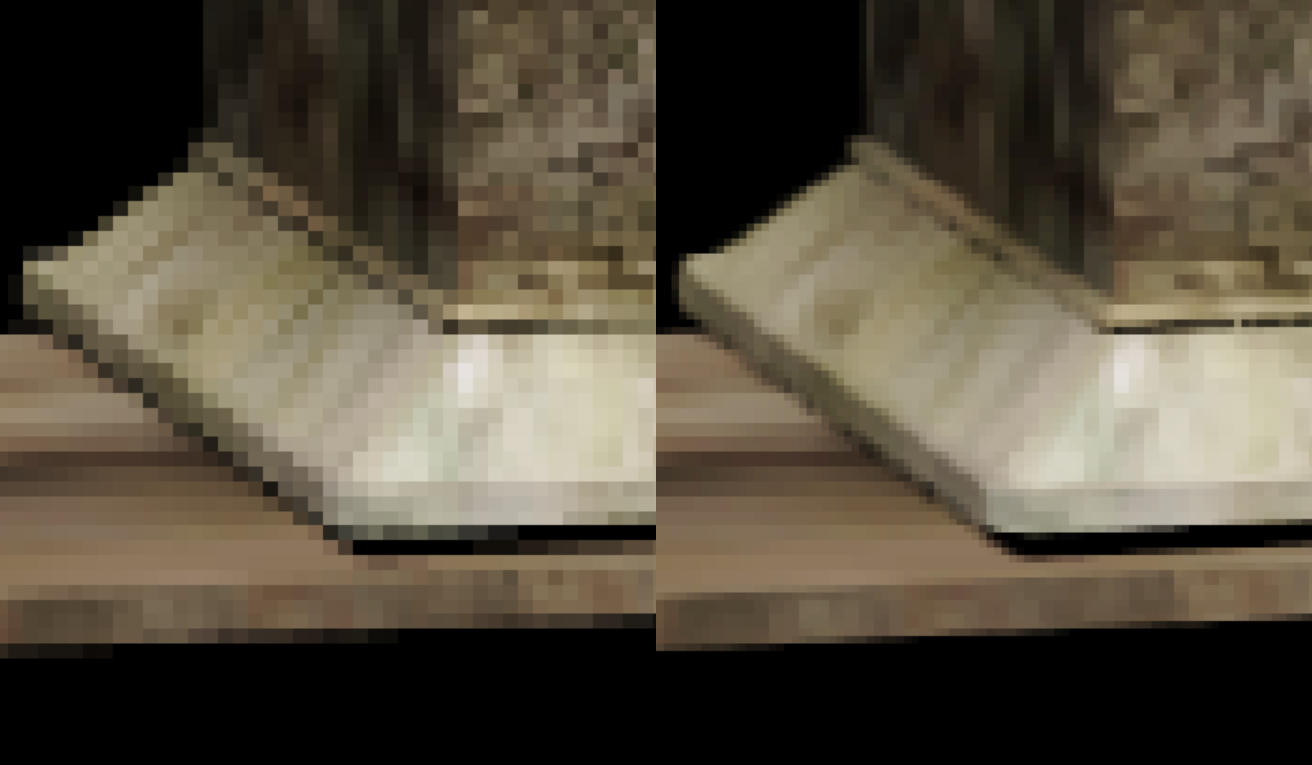
An 8x MSAA image with naive resolve (left) and the upsampled resolve (right).
There is one other thing we can do. We do not necessarily need to use all 16 points for each output pixel. Rather, we can get 4 gradations for each output pixel with only 4 positions as long as these positions solve the N rooks problem.
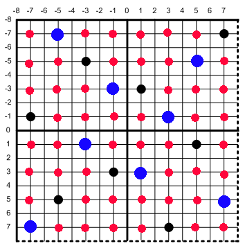
And we can do this by simply swapping out the final pixel evaluation code. Instead of calculating 16 points per pixel, we can get away with only 4. We just keep the two black and two blue points while skipping the 12 red points.
float3 dst00 = (grid__8__9 + grid__9_10 + grid_10_11 + grid_11__8) * (1.0f/4.0f);
float3 dst01 = (grid__8_15 + grid__9_14 + grid_10_12 + grid_11_13) * (1.0f/4.0f);
float3 dst10 = (grid_12_10 + grid_13_11 + grid_14__9 + grid_15__8) * (1.0f/4.0f);
float3 dst11 = (grid_12_14 + grid_13_12 + grid_14_15 + grid_15_13) * (1.0f/4.0f);
Here is a comparison between the two approaches, and there is minimal difference in quality.
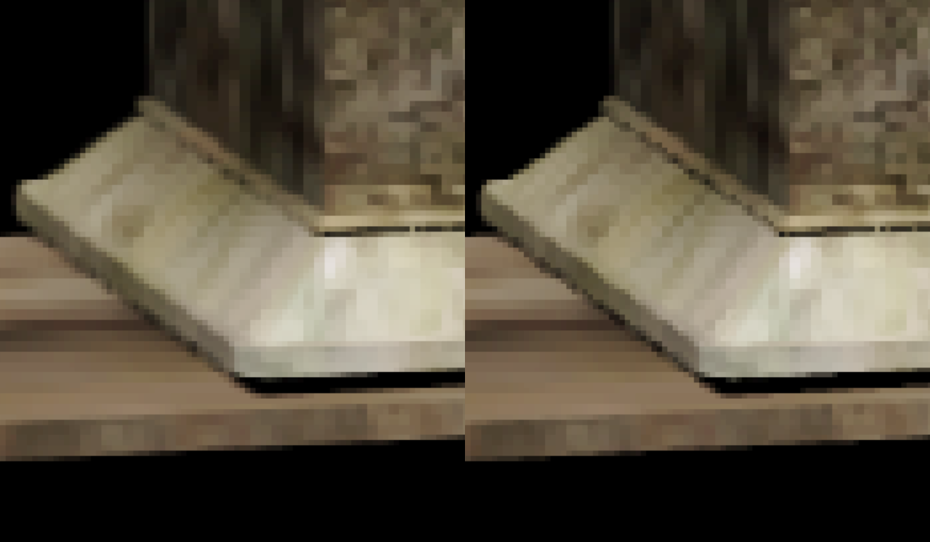
8x upsampling resolve using all 16 samples per output pixel (left) vs using only 4 samples per output pixel (right).
If you look really closely you can see a minor difference, but in general picking “4 rooks” looks very close to brute forcing all 16 samples.
Image Quality
For reference, here is a comparison of all 3 multisample levels.
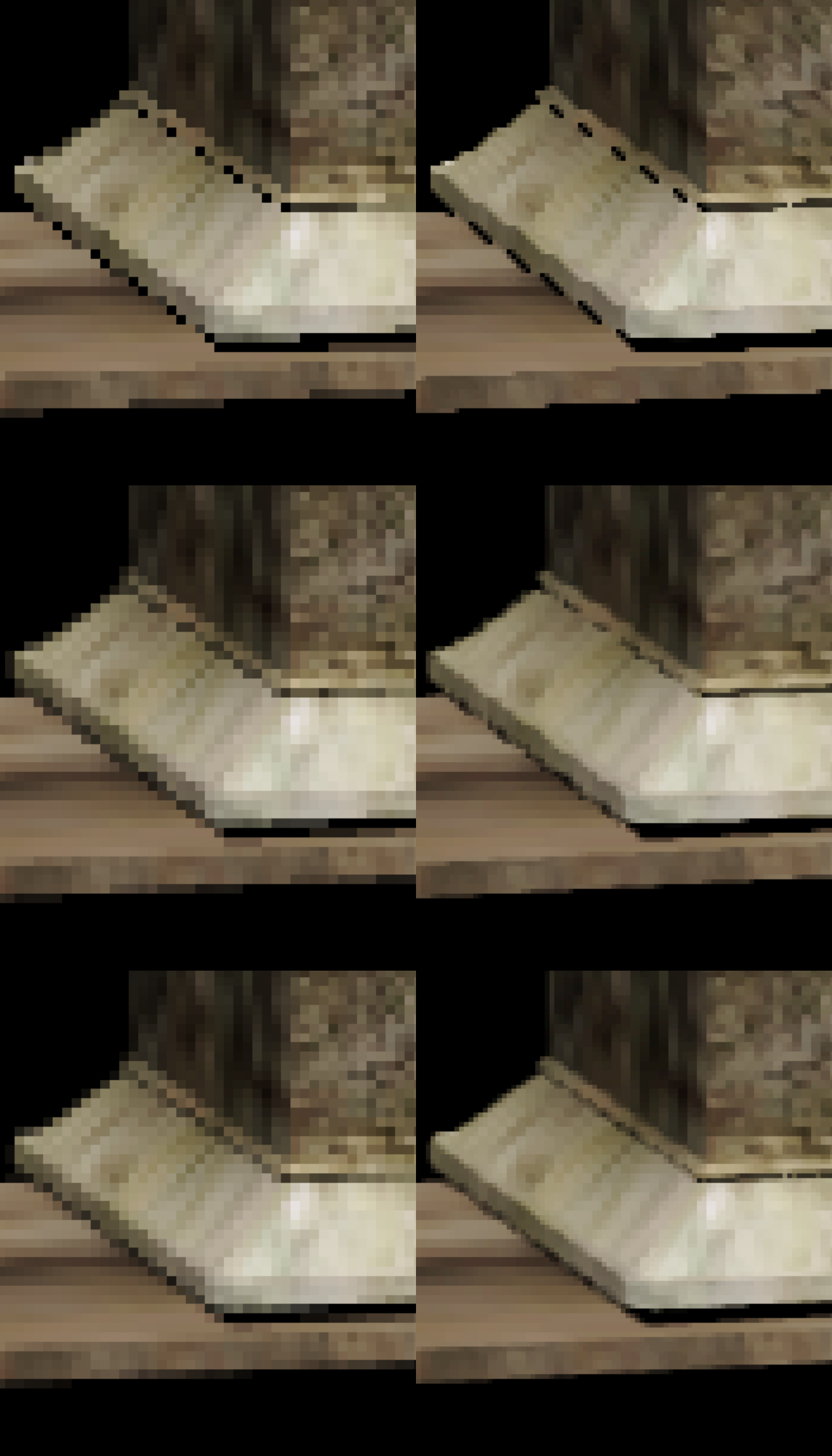
A comparison of 2x (top row), 4x (middle row), and 8x (bottom row) MSAA. In each row, the left side shows the naive resolve and the right side shows the upsampled variation. The 8x upsample uses the 4 rooks approximation.
The first obvious thing to note is that performing an upsample in this method provides no benefit to non-edges. That is because all samples on the same pixel will have the same color. It is possible to use a filter for a mild improvement but that was not done here. How do the long edges look?
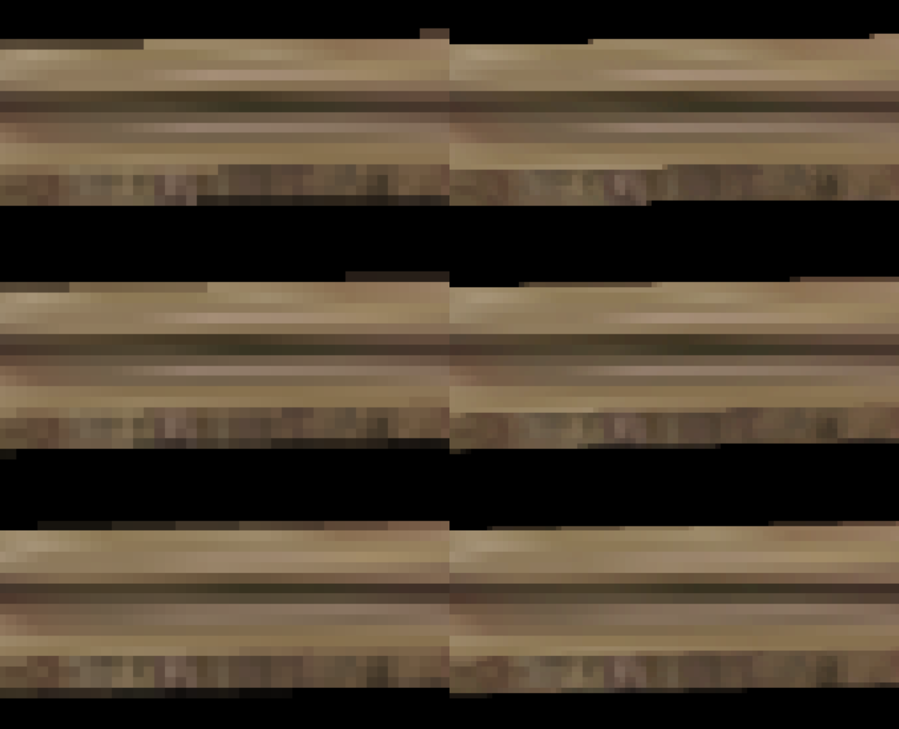
A comparison of 2x (top row), 4x (middle row), and 8x (bottom row) MSAA. In each row, the left side shows the naive resolve and the right side shows the upsampled variation.
In general, the edges look exactly as we would want them to. We would expect a native 4x MSAA image after upsampling to have 2 gradations on the output pixels. Similarly, we would expect the native 8x MSAA image to have 4 gradations in the output pixels. It turns out that both work exactly as we would hope. Let us take a look at another region.
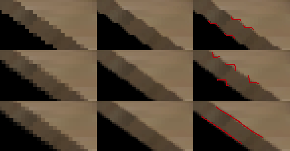
A comparison of 2x (top row), 4x (middle row), and 8x (bottom row) MSAA. In each row, the left column shows the naive resolve and the middle column shows the upsampled variation. The right column is the same as middle but with additional markup.
In the image 2x you can clearly see the “wavy” nature of near-45 degree images. You can see a similar affect in the 4x upsampled image but it is mostly removed once you go to 8x (although if you look really closely you can see slight bending). There are some ways this could be fixed. In particular, it should be possible to write diagonal detection similar to SMAA [10] or MLAA [15], but that was outside the scope of this test. As another option, the Decima Engine [3] actually used FXAA [11] on a rotated diagonal checkerboard image to fix a similar artifact. And if you have not seen that presentation before, it is worth reading through the slides just for the checkerboard tangram trick.
Finally, let us look at some thin lines. While classic sponza does not have any thin lines in it, at the moment alpha testing is broken in this scene (please do not judge me!) so the chains form a beautiful orange line which is perfect for testing.
A comparison of 2x (top row), 4x (middle row), and 8x (bottom row). In each row, the left side shows the naive resolve and the right side shows the upsampled variation.
In this shot, the line on the left is slightly wider than one native pixel, whereas the line on the right is slightly thinner than one native pixel. The upsampling algorithms do a reasonable job with both lines, although we do end up with some jagged teeth. There is a slight gradient in the thin line, but the background is pure black, so the interpolation is choosing the horizontal black gradient which creates little gaps in the line. One way we could address this is using depth, so that if two gradients are very close, we choose the one that is closer to the camera. But this is a problem for another day.
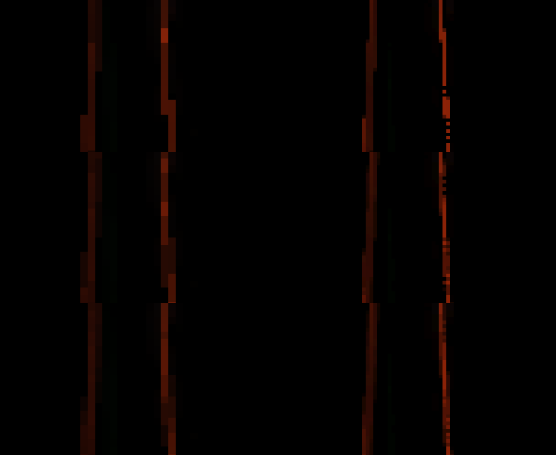
In comparison, this a full failure case for TAA. Since there are frames where the sections of the right line are completely missing, TAA fails to reconstruct the line here. You have probably seen this problem before with thin power lines, fences, and tree branches in the distance.
Thin lines using TAA for reconstruction.
In terms of performance, all times were on my RTX 3070, at 1080p (upsampling to 4k). The code is completely unoptimized, and I would expect significant gains by putting some optimization effort into it. Additionally, the cost would change depending on triangle density, as increased triangle density would mean reading from more image planes in the MSAA target on PC platforms.
| MSAA Level | Upsample Time (in microseconds) |
|---|---|
| 2x | 118 |
| 4x | 283 |
| 8x | 731 |
That being said, the numbers are not particularly meaningful and are just included as a rough starting point. There are many obvious optimizations to make, but the approach for optimization will depend significantly on your platform and use case. Is your platform a mobile TBDR device or a desktop GPU? Are you tonemapping during MSAA resolve? What about depth of field and motion blur? And of course, do you also want to apply a convolution (such as an approximate Lanczos filter)? These numbers are definitely slower than I would like, but there is ample room for improvement depending on the specific use case. Also, there are many options for improving the quality. Temporal reprojection, jittered sampling, and a better filter kernel come to mind just to name a few.
Now, the main problem with this algorithm is that it is only applicable if you are using MSAA rendering. And even then, if you have operations that run in between the main color pass and the final output pass (such as depth of field, distortion, motion blur, bloom, etc) then there are other non-trivial problems to solve. It really is vastly easier to just render everything at 1x with temporal jitter and and use TAA [12], variants of TAA [2], or one of the many upsampling algorithms (DLSS [16], FSR [4], XeSS [13], TAAU [5], GSR [14], ASR [6], etc). But if you do happen to have an MSAA buffer just sitting there in your frame, performing a direct 4x area scale might be a compelling option for you.
Source Code: For a reference implementation, I took these functions and put them into a standalone file with an MIT license. You will have to make minor modifications to get it to work in your codebase (as it was pseudo-ripped out of my larger codebase). But hopefully it can get you started.
UpsamplingViaMultisampling.hlsl
References:
[1] 4K Checkerboard in Battlefield 1 and Mass Effect Andromeda, Graham Wilhidal (https://www.gdcvault.com/play/1024709/4K-Checkerboard-in-Battlefield-1)
[2] A Survey of Temporal Antialiasing Techniques. Lei Yang, Shiqiu Liu, and Marco Salvi. (http://behindthepixels.io/assets/files/TemporalAA.pdf)
[3] Advances in Lighting And AA, Giliam de Carpentier and Kohei Ishiyama. (https://www.guerrilla-games.com/media/News/Files/DecimaSiggraph2017.pdf)
[4] AMD FidelityFX, Super Resolution. AMD Inc. (https://www.amd.com/en/technologies/radeon-software-fidelityfx-super-resolution)
[5] Anti-Aliasing and Upscaling, Epic (https://dev.epicgames.com/documentation/en-us/unreal-engine/anti-aliasing-and-upscaling-in-unreal-engine)
[6] Arm Accuracy Super Resolution, ARM (https://github.com/arm/accuracy-super-resolution)
[7] D3D11_STANDARD_MULTISAMPLE_QUALITY_LEVELS enumeration (d3d11.h). Microsoft, Inc. (https://docs.microsoft.com/en-us/windows/win32/api/d3d11/ne-d3d11-d3d11_standard_multisample_quality_levels)
[8] dcraw.c, Dave Coffin (https://www.dechifro.org/dcraw/)
[9] Experimenting with Reconstruction Filters for MSAA Resolve. Matt Pettineo. (https://therealmjp.github.io/posts/msaa-resolve-filters/)
[10] Filmic SMAA: Sharp Morphological and Temporal Anialiasing, Jorge Jimenez (https://research.activision.com/publications/archives/filmic-smaasharp-morphological-and-temporal-antialiasing)
[11] FXAA, Timothy Lottes (https://developer.download.nvidia.com/assets/gamedev/files/sdk/11/FXAA_WhitePaper.pdf)
[12] High-Quality Temporal SuperSampling, Brian Karis (https://advances.realtimerendering.com/s2014/#_HIGH-QUALITY_TEMPORAL_SUPERSAMPLING)
[13] Intel Arc Gaming Technologies, Intel (https://www.amd.com/en/products/graphics/technologies/fidelityfx/super-resolution.html)
[14] Introducting Snapdragon Game Super Resolution, Qualcomm (https://www.qualcomm.com/news/onq/2023/04/introducing-snapdragon-game-super-resolution)
[15] Morphological Antialiasing, Alexander Reshetov (https://www.intel.com/content/dam/develop/external/us/en/documents/z-shape-arm-785403.pdf)
[16] NVIDIA DLSS. NVIDIA Inc. (https://www.nvidia.com/en-us/geforce/technologies/dlss/)
[17] Rendering Tom Clancy’s Rainbow Six Siege, Jalal El Mansouri. (https://ubm-twvideo01.s3.amazonaws.com/o1/vault/gdc2016/Presentations/El_Mansouri_Jalal_Rendering_Rainbow_Six.pdf)
[18] Variable Number of Gradients (https://web.archive.org/web/20120422035609/http://scien.stanford.edu/pages/labsite/1999/psych221/projects/99/tingchen/main.htm)