
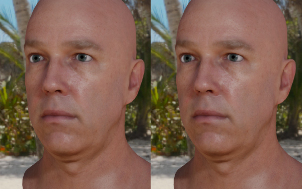
One of the problems that has been bothering me for several years is that it seems like there should be a way to speed up the Fresnel and Visibility functions by combining them together. In particular, Schlick-Fresnel and the Schlick-Smith Visibility term have a similar shape so I’ve done some experiments to combine them together. The results are above with the reference version on the left and the approximation on the right.
To give you an idea of the cost, the per-light code is below and I’ll explain the derivation. The preCalc parameter is derived from roughness and the poly parameter is either from a 2D lookup texture indexed by F0 and roughness or derived from a less accurate endpoint approximation.
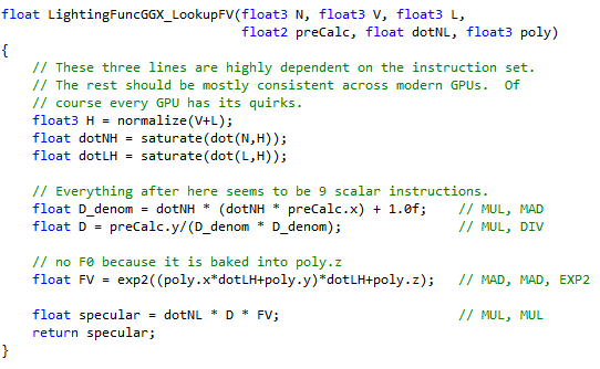
The important thing to note is the FV line. It turns out that if we have a known F0 and Schlick-Smith roughness parameter, the combined function of FV can be modeled with an exponential of the form:
Finally, the full shader source, the example DDS files, and the solver source are included at the bottom of the page under a public domain license.
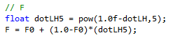
1) Motivation. As you should already know, the most common formula for Fresnel is the Schlick approximation which is:
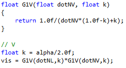
And the Schlick-Smith visibility term uses the code:
At a glance it should not be possible to combine them together. After all, Schlick Fresnel is a function of dot(H,V) whereas visibility is a function of dot(N,L) and dot(N,V). But almost a decade ago I was looking at the MERL BRDF database. The MERL data models isotropic BRDFs using a 3D function of dot(H,V), dot(H,N), and phi (which is the angle between the projected angles of L and V). I did some testing back in 2006-ish and found that you could remove the phi term for most “simple” materials, and just use a 2D function of dot(H,V) and dot(H,N).
That inspired me to create the post last year about combining F and V together by only using dot(H,L), which is the same as dot(H,V) of course. The main idea was to create a 2D texture where you could lookup the lighting function by doing two texture reads per light. Unfortunately it does not help very much because you generally want to avoid dependent textures reads inside your lighting function. You could also use the optimized analytic formula which might save a few cycles because you can ignore the dot(N,L) term. But that does not save much either because you can calculate that value once in the beginning of your shader and reuse it for each light.
But the next inspiration was this post from Sèbastien Lagarde regarding spherical gaussian approximations. That post covers how you can approximate the function:
…with the function…
…where A and B are derived from an optimization procedure and C is zero. That got me thinking: Any function with the same basic shape should have a good approximation using 2 to the power of a polynomial. Since the Schlick-Smith GGX Visibility function has a similar look, we can probably take take the combined Fresnel and Visibility function and solve to it. From here I tried several approaches that all seem to get good results with minor differences.
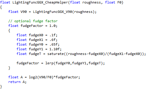
2) Endpoint Matching The first idea is to just get the endpoints to line up. The combined FV function is at a minimum when the light and viewer are at the same position and dot(L,H)=1. In this case, Fresnel is F0, Visibility is 1, and the combined value is F0. The FV function hits its peak at grazing angles and dot(L,H)=0. Fresnel is 1, Visibility is some value which we can call V90, and the combined function is V90. Given some value dotLH, here are the endpoints for our combined FV function. We just need some reasonable function in-between.
We can make this happen with the following function:
C has to be zero because exp2(0)=1. With any nonzero C value our function will deviate from F0. We could optimize B though. As long as B+A=log2(V90/F0) we will hit the correct endpoint, but we will get to that later.
The one obvious issue when trying this function is that some roughness values are too bright. It turns out we do not necessarily want to exactly hit the V90 endpoint. The grazing angles at 80 or 85 degrees are much more visually important than at exactly 90. Thanks to the asymptotic nature of Schlick-Smith with low roughness values this function will overestimate the value at 80/85 to hit that very high V90 value. Going the other way, higher roughness values (like .5 or .6) are too dark. To solve these problems I created a function that tries to get a better perceptual fit for A based on roughness. The code is below as an optional tweak.
3) Linear Solver There are two obvious problems with the endpoint approach. First, while the endpoints match exactly, the middle of the curve does not look quite right. Second, we could use B and C to get a better fit. We can address this using a linear solver.
Given our ground truth function FV(x), we are trying to solve for A, B, and C in the following function:
That function is nonlinear and requires a bit of work to solve. But with a divide and a log we can reduce the function to a simple polynomial:
That function can be easily solved with polynomial curve fitting. Note that while the original function would minimize the squared error, the adjusted function will minimize the squared log error. This is an unexpected benefit since the human eye’s perception of light is logarithmic anyways. Log error squared is probably a better choice than linear error squared.
There are several tweaks that we can perform to optimize the solver. The first question is if we want to constrain C or not. If we let C float around then we will get overall better error but F0 will change. Or we can constrain C and have more error in the middle angles. In my opinion, the constrained version gets a better result but feel free to experiment. The results will also depend on how you weight the samples. It’s simply not possible to get an exact fit so error will have to be somewhere. The problem is finding the least-worst place for that error to go.
Another tweak we can make to the solver is to limit the really strong grazing angles. For the low roughness values the very high grazing angles (88, 89, 90) tend to overpower the lower grazing angles so at roughness 0 we can clamp the angle at 85 degrees. That clamp function lerps so that by roughness .5 the largest angle is back at 90 degrees.
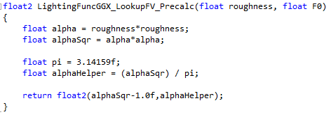
We can also optimize out a few instructions. Our full function looks like this:
First, we can get rid of that F0 term using the following rule:
That removes F0 by adding log2(F0) to C. Also, if we are on a GPU where divide is more expensive than rcp(), we could bake preCalc.y into C as well and replace the divide with rcp().
Second, we can remove the 1-dotLH by plugging the values in and multiplying it out.
Combining all those steps together allows us to calculate a combined FV value in a single exp2() and two fused multiply adds.
The sample code saves the data as a 128x128 texture for roughness and F0. The precision gets a bit low for F0 because dielectric values are between 0.02 to 0.05. So the y axis indexes to F0^2, not F0.
In the final code, you first would calculate your roughness and F0 value. Then apply several small tweaks based on your roughness value to save a few instructions when calculating D.
You would also have to do a table lookup to fetch your polynomial data. Note the sqrt() around F0.
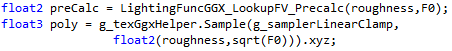
From there you would use this function to accumulate your lighting.
And you would call it like so:

4) Conclusion That should be all the important details of the approximation. I’ve found that the best results come from the constrained solver version. When the dot(L,H) is near one as in this sample it looks nearly exact. You can click on the image for a larger version.

The middle is the reference GGX version, the right is the optimized version, and the left is the difference with levels applied.

When you get near grazing angles the results show a little bit of loss but are still quite acceptable. At grazing angles you can see a difference when you flip back and forth between the reference and the approximation. But if I was looking at a single version by itself I’m not sure if I would be able to tell if it was the reference or the approximation.
With a solver like this, it is interesting to think through how many levels of approximations we are doing. This FV function is not an approximation of the ground truth FV function. Rather, Schlick-Fresnel is an approximation of the ground truth Fresnel function. Schlick-Smith GGX Visibility is an approximation of the true GGX visibility function. So this FV function is an approximation of the product of an approximation and another approximation.
However since we are approximating the function numerically we can easily change the original function and re-solve. If you have a ground truth for both Fresnel and Visibility it would be interesting to solve for those together and see if the result is more accurate than multiplying the approximate Fresnel and approximate Visibility terms together.
We could apply the same approach for any function. There are quite a few functions in computer graphics which have a similar shape and might be well approximated by taking the exp2() of a polynomial. It is trivial to solve to a higher order polynomial if the situation calls for it.
The major downside of this approach is that you do not get F as an intermediary value. If you are conserving energy and want to multiply your diffuse by (1-F) then this approach will not work. It also will not work if your F0 is a color that lerps to white at F90. Technically it will work, but you will have to do it 3 times (one for each channel) which would probably be slower than the reference function.
That being said, there are times when you are really tight on cycles. Mobile systems are becoming graphically comparable to the PS3 and XB360. If we want something better than Blinn-Phong but can not afford full PBR functionality then this approximation might be a good tradeoff. Another application is VR rendering where you have to push a staggering number of pixels per second. High quality VR is going to be tricky even with the most expensive PC that money can buy.
Finally, here is the zip file. GgxPolySolver.zip
It contains:
- Shader code.
- Four variations of the solved polynomial textures.
- C++ source for building these textures</ol> The files are available under a public domain license so feel free to use them however you wish. Please try it out and let me know if you get any good results!