
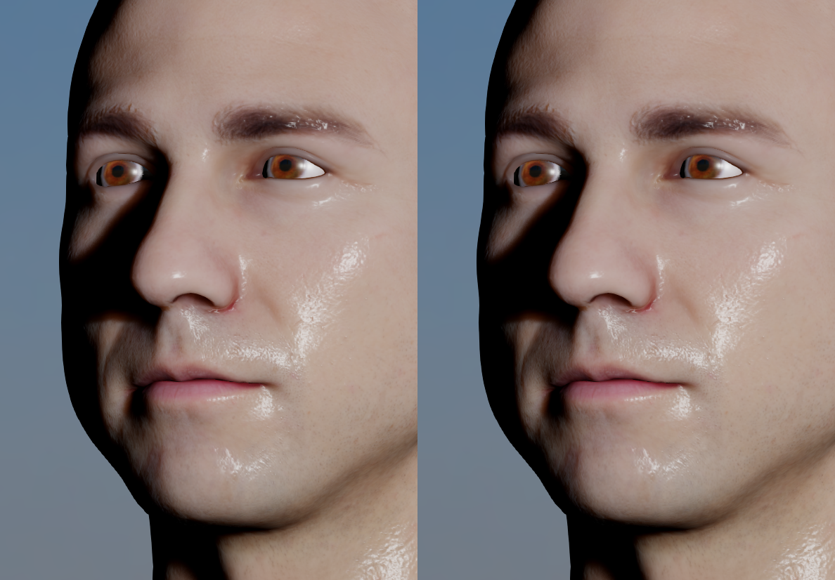
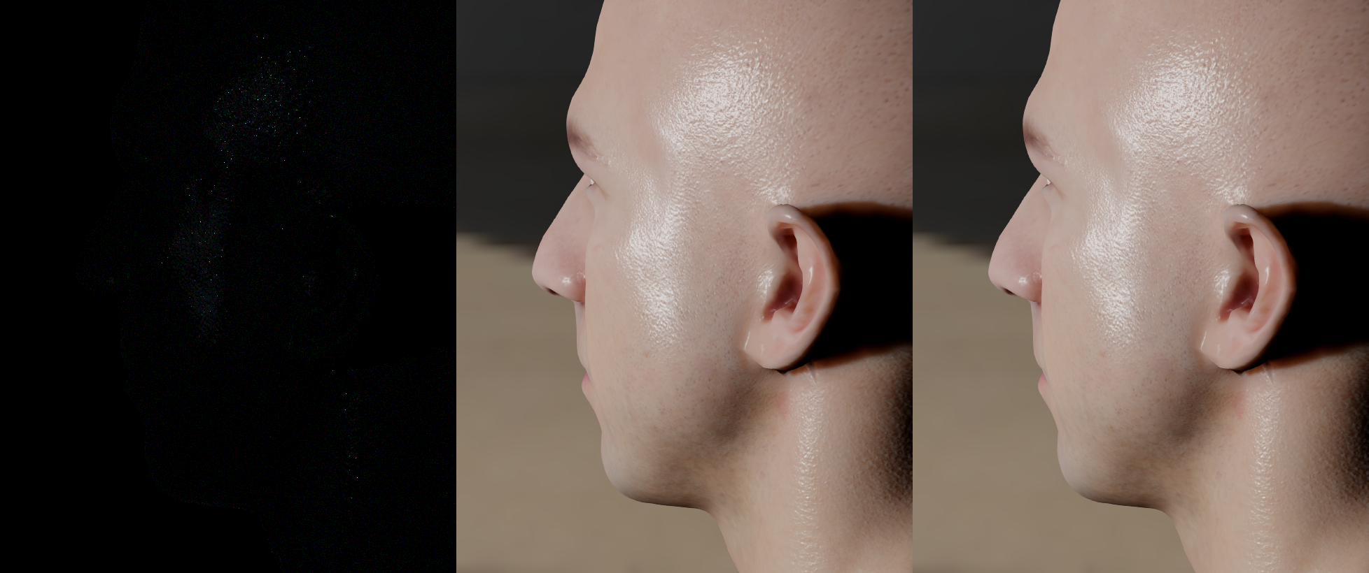
The GGX distribution is quickly becoming the dominant lighting model games. But the obvious downside over the previous models is shader cost. So I’ve been looking at ways of optimizing it and the image above shows the before and after.
The “standard” lighting model takes the Cook-Torrance separation of terms as:
Specular = DFV
And most games are using something along the lines of:
- D) GGX Distribution
- F) Schlick-Fresnel
- V) Schlick approximation of Smith solved with GGX
This approach gives a much better specular term than anything we were seeing last generation. But we have added quite a few instructions so I wanted to see if we can cut it down a bit while still retaining the quality. Spoiler alert: We can do it by doing some tricks with dot(L,H).
Typical GGX Specular Function: There are many places to find code and examples of these functions, but I took the functions from the UE4 Shading presentation by Brian Karis. There are a bunch of good presentations from the Siggraph 2013 Physically Based Shading Course which you can find on Stephen Hill’s website, but the formulas I’m using here came from Brian Karis’s talk. You should also make sure to check out Brent Burley’s talk (“The Disney BRDF”) from the previous year.
In my facial animation talk at GDC, I was still using a distribution based on a bunch of Blinn-Phong lobes, but now that the talk is finished I was able to look more deeply into GGX and I really like the softer tails (just like everyone else).
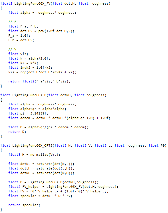
Here is the shader that I’ll be starting with. To make your life easier, I’ll just cut and paste the code. There is a link to all the shader functions at the bottom of the page.
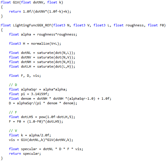
Assuming I didn’t make any mistakes, the formula above is your typical game shader. I’m ignoring the “Hotness Remapping” that Brent Burley mentioned because I prefer the look of the hot highlights, but you can go either way. Now, let’s start optimizing.
Visibility Functions:
Ideally, I would like to come up with something that is close to Schlick-Smith, but cheaper. There are several other options for the visibility term. But the one that interests me the most is the Kelemen-Szirmay-Kalos approximation of Cook-Torrance as described in the Siggraph 2010 course by Naty Hoffman.
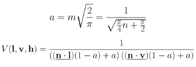
Before we get too far ahead, let me apologize in advance for taking screenshots of different presentations with different notation. In the image below, the entire left side is just the Visibility term V.
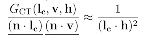
The nice thing about this function is that it is very cheap, but the problem that was mentioned several times is that it is too bright. But why?
When I think of lighting functions, I think about the endpoints. The KSK visibility term is lowest when dot(L,H) is one and is highest when dot(L,H) is zero. Note that since H is the half vector between L and V, dot(L,H) and dot(V,H) are the same thing, so don’t get confused if I say dot(L,H) but the formula says dot(V,H) (or vice-versa).
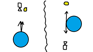
The image above shows the high and low cases for KSK visibility. Coincidentally, these are the same as the high and low cases for Fresnel. If the light and the camera are pointing straight at the normal, then the V term is 1.0. But as you get towards grazing angles the V term goes to infinity. In reality, you don’t actually get to infinity because the entire function is modulated by dot(N,L). That would explain why the Black Ops team thought that KSK was too bright in their talk on on Physically Based Shading in Black Ops.
What does Schlick-Smith look like for GGX?
First off, I’m going to refer to that a parameter as k. So, what do the extremes look like? When you are straight on (N=V=L), it is 1.0 just like KSK or Cook-Torrance. But when you go to grazing angles it converges to 1/(k^2), since dot(N,L) and dot(N,V) both go to zero.
That makes sense. KSK and Cook-Torrance say that every single surface’s visibility term goes to infinity at grazing angles. But Schlick-Smith says that the visibility term converges to 1/(k^2). And k is a value that increases as roughness increases, so smoother surfaces have brighter grazing angles than rougher surfaces.
The brightness of grazing angles is an interesting question. In the Disney BRDF used in Wreck-it-Ralph, they remapped the k value in the V function to make it “less hot”. There is no physical basis for this decision, rather they changed it to fit the artistic style.
Ultimately, we don’t actually know how bright grazing angles are supposed to be. It’s strange but true. To me, 1/(k^2) seems like a perfectly valid value, and remapping the range is valid as well. Unfortunately, the MERL data does not have reliable data at those grazing angles so we just don’t know. In my opinion, any reasonable V function that gets brighter as the surface gets smoother is probably fine.
But infinity is probably too high, which explains why KSK and Cook-Torrance are too bright at grazing angles. They don’t account for the increased microfacet self-shadowing of rougher surfaces. But is there a way we can get the same effect with a cheaper function?
We can do this by replacing both dot(N,L) and dot(N,V) with dot(L,H). Let’s think about our two main cases: Straight ahead and at a grazing angle. In both cases, the specular peak will happen when the V vector reflects directly into the L vector. Which means that H=N. So we can just replace the old V term:
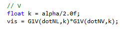
with this new V term:
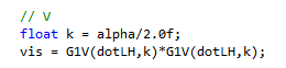
And it should look really close. We can go farther than that though. Ultimately, all I want is a function that goes to 1 when at direct angles and goes to 1/k^2 at grazing angles, so we can optimize it further as this:
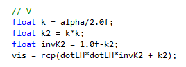
An intuitive way to think about this approximation is that the original function calculates the visibility amount once for dot(N,V), and then again for dot(N,L). Instead we can just split the difference using dot(L,H), and use that value for both sides.
One more note: This isn’t a new idea. In the Black Ops 2 Specular presentation, they optimized the function using k=min(1,gloss+0.545). The difference is that I’m treating the 1/k^2 as the explicit V function at grazing angles, 1 as the explicit function at at direct reflectance, and just doing something reasonable in the middle. What I prefer about this function is that at every glossiness value you get some brightening at grazing angles, and that grazing angle brightness gradually increases as roughness decreases.
So that’s a nice little win. We don’t need to calculate dot(N,V). It saves a few instructions, which I’ll take. But there is a lot more we can do.
Look Up Tables The really interesting thing is that now V and F are both based on dot(L,H). So we should be able to combine them together and think of them as a single, combined formula FV. For reference, here is the Schlick approximation of Fresnel:
Note that when the formula says R0, I mean F0.
It’s relatively straightforward to turn the Visibility term into a lookup. The two parameters are dot(L,H) and roughness. That’s a 2d texture. But F is a little tricker. First, F0 can be a scalar, so if we want to calculate V and F together, that would need a 3d texture indexed by (dotLH,roughness,F0). That can get pretty big pretty fast. Also, sometimes you need a specular color, so we would have to do 3 lookups for each channel (R, G, B).
But there is a nice little trick. The fresnel term has a left side which is multiplied by F0, and a right side which is multiplied by (1-F0). So we can return both values in the table, and do the F0 lerp in the shader.
The GGX distribution function is also quite simple to do in a table. We just need dot(N,H) and roughness.
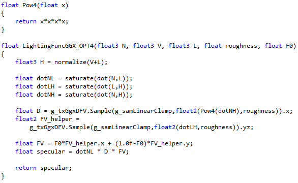
Here is the refactored shader:
All that’s left is to switch the internal functions to texture lookups and we’re done. There is one more gotcha, which is that dot(N,H) has terrible precision. For tighter specular functions, the cosine of the angle stays near 1.0 and is very slow to fall off. So we should take those cosines to a power (in this case 4) so that they fall away from 1.0 faster and give us better precision. In my case, I went with a BC6h texture that is 512 wide by 128. We could also take it to a higher power (square it again?) which would let us drop it by 512 into something lower.
It would be nice to make that texture smaller, and there are a few ways we could do it.
- Use the analytical formula for low roughness values with a shader switch or something like that.
- Use a higher power on the cosine.
- Do not have low roughness values.
- Deal with it. The MERL data set measures all three angles to a resolution of one degree. In very sharp highlights there is some falloff happening in that one degree, but for console games we can probably just let it go.
Here is the final shader:
In terms of accuracy, it is very close. You will see some precision loss for low roughness values if your texture is not large enough. But otherwise it looks good enough for me. Here are some comparisons. The left image is the diff with a levels (0-64) on it in Photoshop. Middle is the original, and Right is the texture lookup approximation.
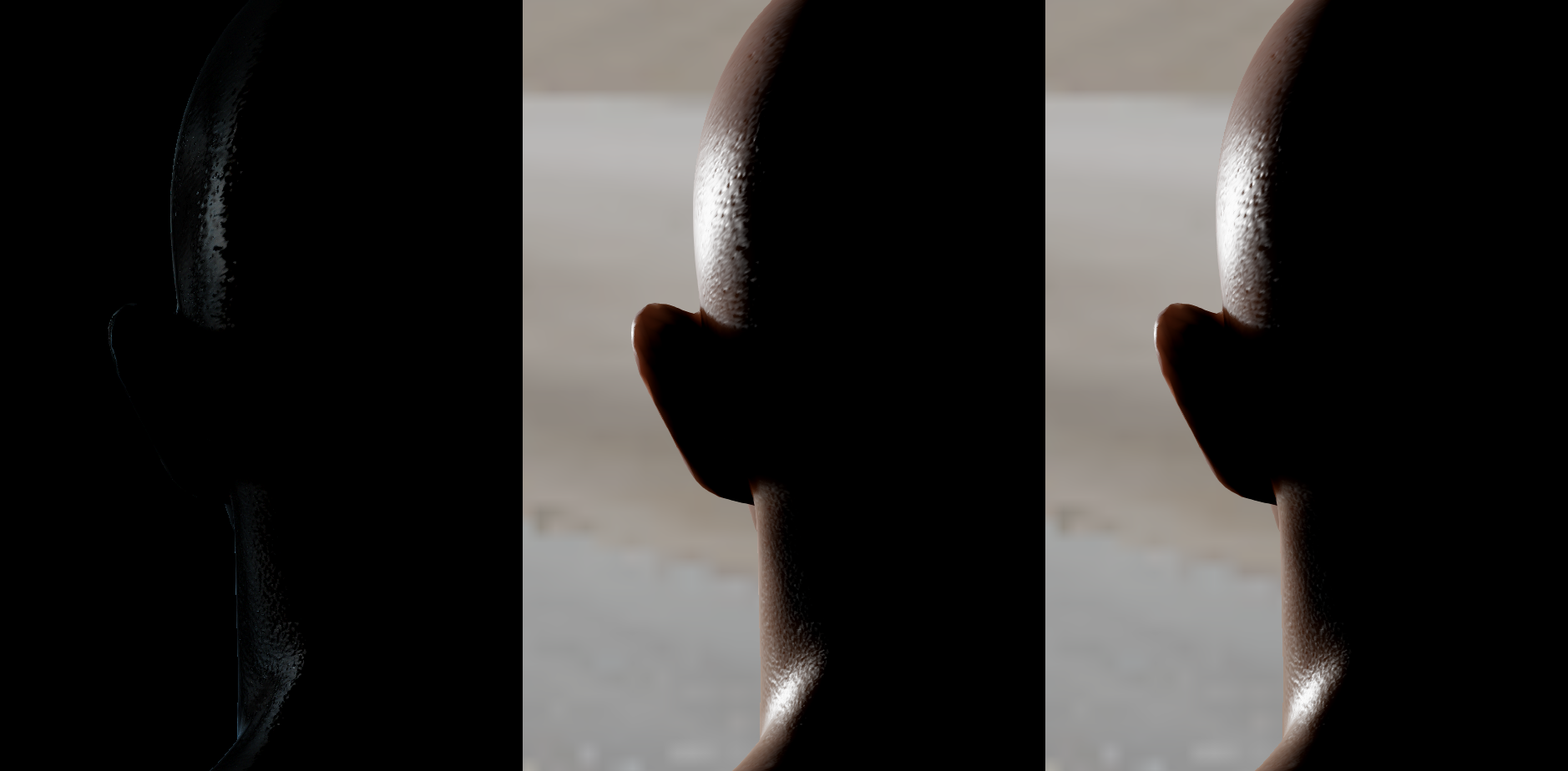
Here is another example. It’s the same thing except the levels on the diff goes is from (0-16). Otherwise you can’t see anything in the diff.
In terms of performance, will this actually help? It depends. The initial trick of switching out dot(N,L) and dot(N,V) with dot(L,H) should always be a win, because it is one less dot product. Performance for a texture lookup will vary considerably. If you are primarily ALU bound, it should help. But if you are doing it in a pass that is already bandwidth and texture sampler bound, it will hurt. I can’t tell you which version is better, since the only real solution is to test it out.
There are other things we can do as well. In Brent Burley’s presentation he looked at the 2D slices of BRDFs. These slices show one axis as the angle between (L,H) and the other axis as the angle between (H,N). The slices shown in the presentation correspond to phi=0, meaning that L,V,N are all coplanar. If we were to fix the roughness term and the fresnel F0, we could combine the whole function into a single 2D slice.
Finally, here is the source shader file. The license in the shader file states that everything in there is public domain, so feel free to use it any way that you wish.