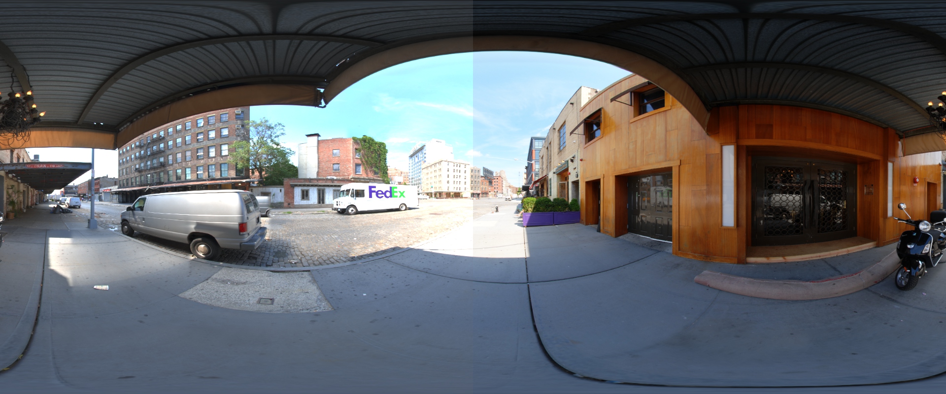
It’s been a long while since the original posts on Filmic Tonemapping, and it is time for an update. For newcomers, the basic premise of Filmic Tonemapping is to simulate the tone curve of film in our images, with a shoulder and a toe. In the image above, the left side is a pure linear tonemap and the right side uses a filmic curve.
For a little history, the orignal curve was authored as an approximation to the Kodak response curve by Haarm-Pieter Duiker (@hpduiker). The presentation is actually online at HP’s website: Filmic Tonemapping and Color In Games. He used the Cineon linear to log node to convert from linear to log and then applied a LUT for the final look. Then he ported it into an hlsl shader. While HP and I were at EA on the LMNO project, Jim Hejl (@jimhejl) and Richard-Burgess Dawson found a faster approximation using ALUs which made the process more practical on PS3 and XB360. After moving to Naughty Dog I was a huge believer in Filmic Tonemapping and ended up getting it into the game, but the Uncharted franchise has a hyper-realistic look so I hacked Jim and Richard’s formula to give some measure of control.
There are plenty of ways to author a look and bake out the LUT, such as Waylon Brinck’s Siggraph 2016 Talk (Technical Art of Uncharted 4). That’s a great option if your artists are comfortable working in offline editing tools and you have the infrastructure to easily roundtrip screenshots back into the tool you are using to author the look (Fusion in this case). But I’ve found that many people are still using the Uncharted 2 curve because of its simplicity to integrate.
This post is an attempt to fix that. Off and on for the last few years I’ve been iterating on a simpler method to author Filmic Tonemapping curves in engine. There are several specific issues I’m hoping to address from the Uncharted 2 curve:
- Simple intuitive controls: Controls should be simple and easy to understand for artists.
- Direct control over dynamic range: This issue was a big one for me. Using the Uncharted 2 curve is "all or nothing". It's not possible to make a plain linear curve using those controls. There are times where you want a plain linear curve with a slight shoulder (like on foggy days) and times where you need to heavily compress the highlights and shadows (like direct sunlight).
- Well behaved curves: The Uncharted 2 curve has weird behaviour if you push the parameters. The new formula lets you go all the way to linear and back without weird behavior or concavity changes.
- Controls in engine: The new curve should only use simple linear parameters and not require going back and forth with a curve editor.
- Fast, closed form: The curve should be simple and fast to evaluate. The exact cost does not matter much because we can bake to a LUT these days, but the cost of baking that LUT should be reasonable.
- Lerpable parameters: In games we often need to have different curves in different areas with a clean blend between them. We should be able to lerp the input parameters and have a reasonable transition between the two curves.
- Simple inverse: Due to engine constraints we need to sometimes calculate the inverse for post effects.
- Convolve with output gamma: It would be nice to have the option to convolve the output gamma into the curve. It turns out we can do that.
- Code on Github: Makes integration simple. Source is available under a permissive license (CC0). You can find it here: github.com/johnhable/fw-public.
A filmic curve has three parts, a linear section, a shoulder, and a toe. The short version is that a toe gives you crisper blacks, a shoulder gives you a softer transition to your overexposed highlights, and the linear section should look relatively unchanged. For a more complete explanation I’d recommend this post on Film Contrast Characteristics.
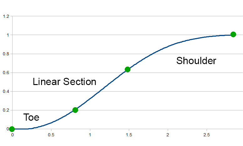
We can think of the curve as three separate segments from four points. The first point is at the origin (0,0). The second point marks the transition from the toe to the linear section, and the next point marks the transition from the linear section to the shoulder. Our last point is the white point of our curve.
When looking at the image, what I realized is that we effectively have 5 parameters. The first point has no parameters because it is always at the origin. And the last point is always at y=1 so we only need a parameter for X. We have the (x0,y0) pair for the start of the linear section, the (x1,y1) pair for the end of the linear section, and a white point (W). Then we can find a reasonable curve to interpolate those values and we are done.
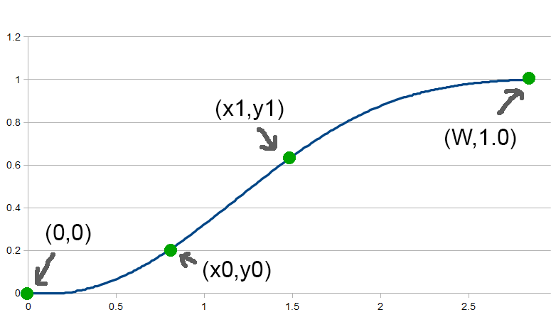
It might seem a little weird that we do not need to describe any parameters for the toe, but it is described implictly by the (x0,y0) parameters and the slope of the linear section. As long as the toe function matches the position and slope of the (x0,y0) curve, the toe should behave as we would expect. The same effect happens for the shoulder.
We’re actually going to have a level of indirection here. One catch is that the parameters do not behave nicely when moved separately. For example, if we want a longer or shorter toe, we usually want to move (x0,y0) together. So we’ll first describe the Direct Curve where the parameters are (x0,y0,x1,y1,W) and a few more. Then we’ll describe a level of indirection with User Params where artists can specify intuitive parameters (like Toe Strength) and derive the Direct Params.
Part 1: Direct Params with Power Curves
Given those points, how can we form a continuous curve between them? One option would be polynomials, but that does not work well. These changes can be pretty sharp in linear space and fitting to polynomials will sometimes have undesirable concavity changes. Instead, we are going to use power curves.
The base curve that we will use is:
y = Ax^B
That curve will actually have problems with floating point precision (as B increases, A gets exponentially large/small and can go FLT_MIN/FLT_MAX). So our curve segment will actually be:
y = e^(ln(A) + B*ln(x))
Note that ln(A) is a constant. It is just a different way of rewriting the power curve. Finally, we need to apply an offset and scale so the actual curve will be:
y = scaleY * e^(ln(A) + B*ln((x - offsetX) * scaleX)) + offsetY
We need the separate scaleX and scaleY parameters in order to flip the curve left to right and upside down. Each of our three segments (shoulder, linear section, and toe) will be a curve of that form. Then to evaluate the curve in the shader or on CPU, the formula is:
float FilmicToneCurve::FullCurve::Eval(float x) const
{
	int index = (x < m_x0) ? 0 : ((x < m_x1) ? 1 : 2);
	CurveSegment segment = m_segments[index];
	return segment.Eval(x);
}

float FilmicToneCurve::CurveSegment::Eval(float x) const
{
	float x0 = (x - m_offsetX)*m_scaleX;
	float y0 = expf(m_lnA + m_B*logf(x0));
	return y0*m_scaleY + m_offsetY;
}
That code skips some of the details, but the key idea is we can represent the filmic curve as three power segments. To evaluate the full curve we can just figure out which segment we are on and calculate the value.
Deriving the Linear Section
Describing a linear section is pretty easy. That section is an offset and scale where B=1.0. Done. It will actually get slightly more complex when we want to conolve gamma though.
Deriving the Toe
Fitting the toe is quite simple as well. Ignoring the offset and scale, we want to find a function with the following constraints:
- It goes through the origin.
- It meets the linear section at the same point.
- It matches the slope of linear section at the same point.
So given our function and its first derivative:
f(x) = Ax^B
f'(x) = ABx^(B-1); // derivative of f w.r.t. x
The formula is:
// find a function of the form:
//   f(x) = e^(lnA + Bln(x))
// where
//   f(0)   = 0; not really a constraint
//   f(x0)  = y0
//   f'(x0) = m
static void SolveAB(float & lnA, float & B, float x0, float y0, float m)
{
	B = (m*x0)/y0;
	lnA = logf(y0) - B*logf(x0);
}
Note that we are finding the log of A, instead of A directly.
Deriving the Shoulder
For the shoulder, we can do the same thing as the toe except flip it horizontally and vertically. We end up with a problem though.
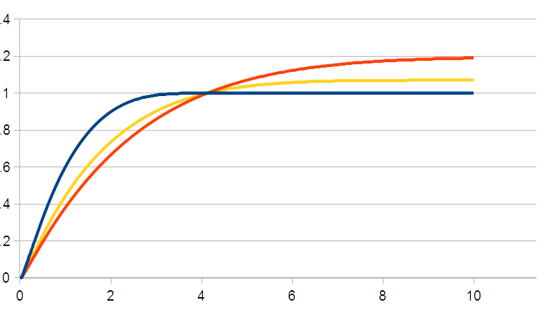
When I first implemented this function, I thought I had a bug in my code. The flipped power function is nice because it guarantees that we will get closer and closer to 1.0 without actually hitting it until our desired white point (W). The catch is that it is so close to 1.0 that it is not meaningful.
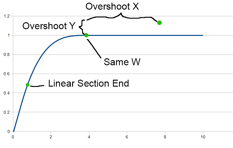
Here is a graph of the sample curve. It is supposed to hit white just after a linear value of 4.0, but perceptually it seems to hit white earlier. That’s becuase at value 3.25, it hits 0.996 after converting to gamma space, which is our last 8 bit value. So the entire range from 3.25 to 4.00 goes from an output of 254 to 255. That is not very useful, and we would like a curve that is not quite as flat.
Instead, we are going to Overshoot the white point. We are going to add two parameters, overshootX and overshootY. Instead of having the power curve end at (W,1.0), it will end at (W + overshootX,1.0 + overshootY). By changing how far we overshoot, it will increase the angle and give us more range at the end of our shoulder.
This change adds an additional complication though. Since we are overshooting, we are not guaranteed to hit the white point at our expected value of W. We could choose either overshootX or overshootY, and derive the other parameter such that we hit 1.0 at our chosen white point. But it is messy function that does not have a closed form as far as I can tell. Instead, we can apply a scale to the overall function at the end to fix it.
Here is the same curve with several different values of overshooting. Note that we end up changing the linear section slightly because of the scaling to make sure that we hit white at W.
Scaling the function.
There are a few more tricks we can do. To simplify things, we can scale all of our x values by 1.0/W. I.e. scale it so that we hit white at 1.0. This operation makes it simpler to bake the function into a texture.
Convolving gamma.
Finally, we can convolve a gamma parameter into the function. Our filmic curve takes a linear value as input and outputs a linear value as output, but in many cases we would want to apply display gamma to it. We can do that by tweaking our input parameters slightly.
Using the tools listed above, from our intial parameters we can derive a filmic curve that for sake of clarity we can call F(x). Then in most cases we want to apply a gamma function. Let’s call it G(x). And the combined function is H(x).
F(x) = // our filmic function
G(x) = pow(x,displayGamma). // gamma correction
H(x) = G(F(x)) // our filmic function, followed by gamma.
Also, we know that our filmic function has the following constraints:
F(x0) = y0
F(x1) = y1
F'(x0) = m
F'(x1) = m
Using the chain rule, we know:
H(x) = G(F(x))
H'(x) = G'(F(x))*F'(x)
And our constraints in the middle of the curve become:
H(x0) = G(y0)
H(x1) = G(y1)
H'(x0) = G'(y0)*m
H'(x1) = G'(1)*m
So if we want to combine the filmic curve with a gamma step, we can just apply the chain rule to our starting points and solve the function. Note that it is not a perfect approximation, and there is no reason to do this if you are baking to a LUT anyways. But if you find that you need to do both steps in the shader and you can not use a LUT for whatever reason you have that option.
One last thing: After convolving with a gamma curve our linear section is no longer linear. But since our function has an offset and scale built into it that is not a problem.
Inversion
A final fringe benefit of this function is that its inverse is of the same form. For a curve segment, the inverse is very similar to the normal evaluation.
float FilmicToneCurve::CurveSegment::Eval(float x) const
{
	float x0 = (x - m_offsetX)*m_scaleX;
	float y0 = expf(m_lnA + m_B*logf(x0));
	return y0*m_scaleY + m_offsetY;
}

float FilmicToneCurve::CurveSegment::EvalInv(float y) const
{
	float y0 = (y-m_offsetY)/m_scaleY;
	float x0 = expf((logf(y0) - m_lnA)/m_B);
	return x = x0/m_scaleX + m_offsetX;
}
In summary, here are the params that control this curve:
float m_x0;
float m_y0;
float m_x1;
float m_y1;
float m_W;

float m_overshootX;
float m_overshootY;

float m_gamma;
- (x0,u0) and (x1,y1) define the linear section.
- W defines the white point.
- overshootX and overshootY add extra space to allow for a steeper shoulder.
- gamma is an extra gamma to convolve into the curve.
Part 2: User Params
The curve listed above is a method of choosing specific points on a graph and deriving a smooth filmic tonemapping curve from it. The catch is that these parameters are unintuitive to control for an artist. Making the curve act differently in a useful way often requires moving several parameters together. For example, if you want to move dynamic range from the linear section to the shoulder, you need to move both (x1,y1) together. That is because you would want to move the point along the linear section as opposed to tweaking x and y separately.
Another problem is that you can end up with bad parameters. As an example, you always want the toe to have positive concavity and the shoulder to always have negative concavity. Ideally the parameters should be defined such that these cases are guaranteed.
So we are are going to use a different set of controls that intuitively describe the curve (like how strong the toe is, how long the shoulder is, etc). Then we will derive the direct parameters for the curve.
These are the parameters that we will expose to artists:
float m_toeStrength; // [0-1]
float m_toeLength; // [0-1]
float m_shoulderStrength; // [0-1]
float m_shoulderLength; // in F stops
float m_shoulderAngle; // [0-1]
float m_gamma;
To derive our direct parameters, we will need to limit the curve in a few ways. The first simplification is that we are going to force the linear section to always have a slope of 1.0. At first this might seem like a problematic limitation, but in reality we do not lose much generality. It is implied that before applying this curve, you are going to perform an exposure adjustment. I.e. you will multiply the entire light intensity by a value. Shifting the slope of the linear section is equivelent to using a slope of 1.0 with an exposure adjustment.
In the past I have tried using a separate control for the slope of the linear section, but then the controls for the linear section and the toe are always fighting each other. So the most reasonable fix is to lock the slope of the linear section. There might be better ways, but after experimenting that seems like the best tradeoff.
Toe Params
We have two toe params, toeStrength and toeLength. The length affects how much of the dynamic range is in the toe. With a small value, the toe will be very short and quickly transition into the linear section, and with a longer value having a longer toe. The formula is simply:
x0 = toeLength * .5;
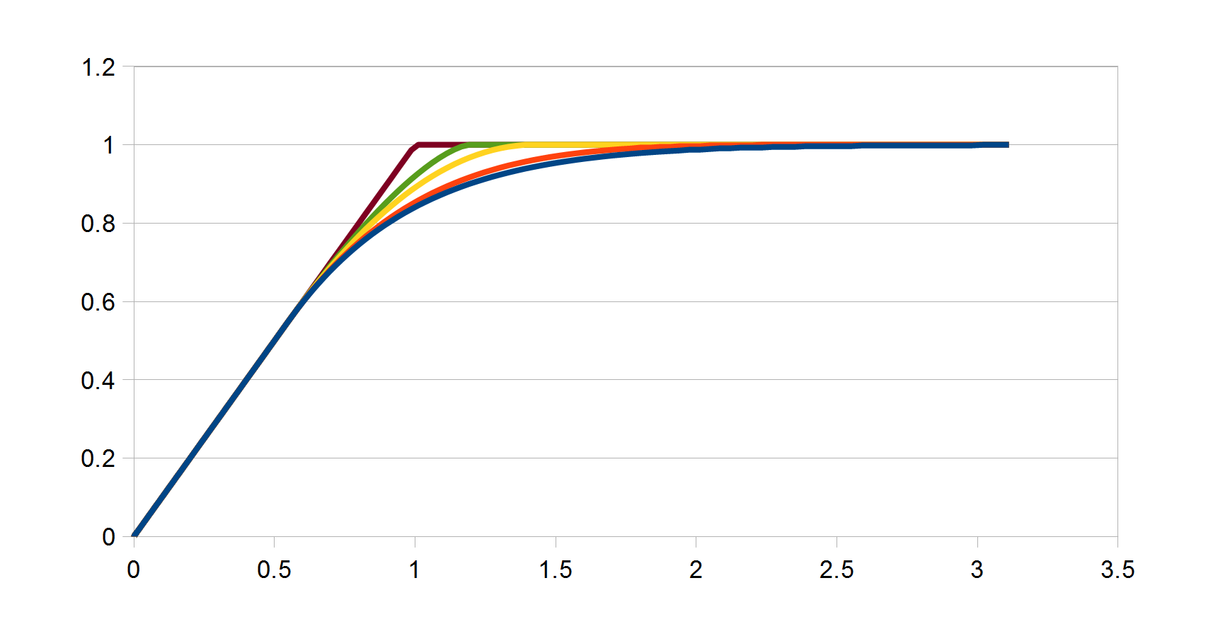
A value of zero means no toe, and value of 1 means the toe takes up half the curve. In the graph below, the blue curve is just linear because it has no toe. The next curve over (orange) has a slight toe, all the way to the purple line which has a long toe. Ths parameter affects how quickly the toe transitions to the linear section.
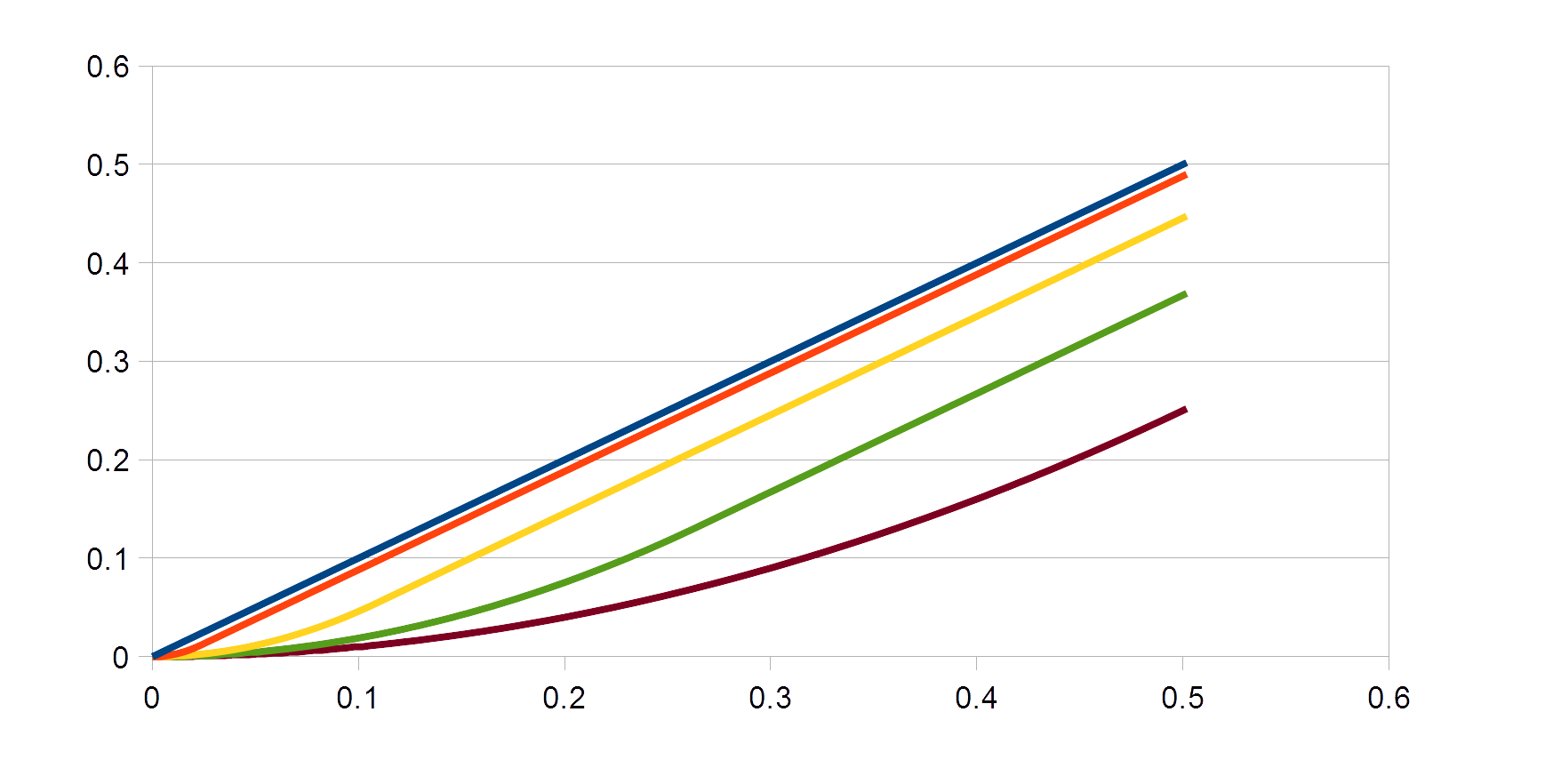
Toe Length
The toe strength param drops the y0 param resulting in a stronger toe. We just use it to lerp y0 between x0 and 0. Note the toe transitions to the linear section at the same point x coordinate in all 5 curves (0.11). In the extreme case (purple) the toe is completely flat against the x-axis.
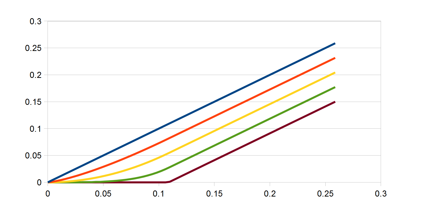
Toe Strength
Note that there are two ways to disable the toe. By either setting toeLength or toeStrength to 0 the toe will disappear, but in general it is best to leave the toe length at a constant value and adjust using only toe strength.
Shoulder Params
We have three shoulder params: shoulderStrength, shoulderLength, and shoulderAngle.
The shoulderStrength param intuitively affects where the shoulder curve starts in the graph. After we have our (x0,y0), shoulderStrength determins both (x1,y1). If shoulderStrength is 1, it means that the shoulder starts right where the toe ends (i.e. y1=y0) and the shoulder takes as much range as possible. If shoulderStrength is 0, then y1=1 and there is no shoulder.
The next graph shows several values of shoulderLength. It is a little hard to see, but all 5 curves (except the linear one) end at the same white point. However all the curves have a different transition point from from the linear section to the shoulder.
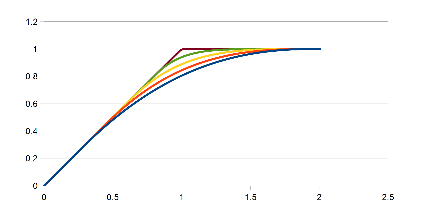
Shoulder Length
The shoulderLength parameter describes how many F stops we want to add to the dynamic range of the curve. Wherever we would hit white if shoulderStrength were 0, we add that many F stops to our linear white value (W).
Th next graph shows the shoulderStrength parameter. The shoulder transitions from the linear section at the same point in all three curves. Each of the three curves hit white at different points. The blue curve actually has a much higher white point than the previous one (orange) but they get packed together because no overshoot is enabled in this graph.
Shoulder Strength
Finally, shoulderAngle describes how much overshoot to add to the shoulder, and more overshoot causes a steeper angle. There is not much science behind this formula, but it seems to work well.
m_overshootX = (W * 2.0f) * shoulderAngle * shoulderStrength;
m_overshootY = 0.5f * shoulderAngle * shoulderStrength;
Perceptual Gamma
Since the entire curve is in linear space we will need to allow the artists to easily define very small values. As a simple trick, we can apply a power of 2.2 to toeLength to allow finer control of the toe.
Convolved Gamma
Finally, the we pass through the convolved gamma. Nothing to see here.
User Params to Direct Params
Here is the full function to convert from the user supplied parameters to the direct curve parameters.
void FilmicToneCurve::CalcDirectParamsFromUser(CurveParamsDirect & dstParams, const CurveParamsUser & srcParams)
{
	dstParams = CurveParamsDirect();

	float toeStrength = srcParams.m_toeStrength;
	float toeLength = srcParams.m_toeLength;
	float shoulderStrength = srcParams.m_shoulderStrength;
	float shoulderLength = srcParams.m_shoulderLength;

	float shoulderAngle = srcParams.m_shoulderAngle;
	float gamma = srcParams.m_gamma;

	// This is not actually the display gamma. It's just a UI space to avoid having to
	// enter small numbers for the input.
	float perceptualGamma = 2.2f;

	// constraints
	{
		toeLength = Saturate(toeLength);
		toeStrength = Saturate(toeStrength);
		shoulderAngle = Saturate(shoulderAngle);
		shoulderLength = Saturate(shoulderLength);

		shoulderStrength = MaxFloat(0.0f,shoulderStrength);
	}

	// apply base params
	{
		// toe goes from 0 to 0.5
		float x0 = toeLength * .5f;
		float y0 = (1.0f - toeStrength) * x0; // lerp from 0 to x0

		float remainingY = 1.0f - y0;

		float initialW = x0 + remainingY;

		float y1_offset = (1.0f - shoulderLength) * remainingY;
		float x1 = x0 + y1_offset;
		float y1 = y0 + y1_offset;

		// filmic shoulder strength is in F stops
		float extraW = exp2f(shoulderStrength)-1.0f;

		float W = initialW + extraW;

		// to adjust the perceptual gamma space, apply power
		dstParams.m_x0 = powf(x0,perceptualGamma);
		dstParams.m_y0 = powf(y0,perceptualGamma);
		dstParams.m_x1 = powf(x1,perceptualGamma);
		dstParams.m_y1 = powf(y1,perceptualGamma);
		dstParams.m_W = W;

		// bake the linear to gamma space conversion
		dstParams.m_gamma = gamma;
	}

	dstParams.m_overshootX = (dstParams.m_W * 2.0f) * shoulderAngle * shoulderStrength;
	dstParams.m_overshootY = 0.5f * shoulderAngle * shoulderStrength;
}
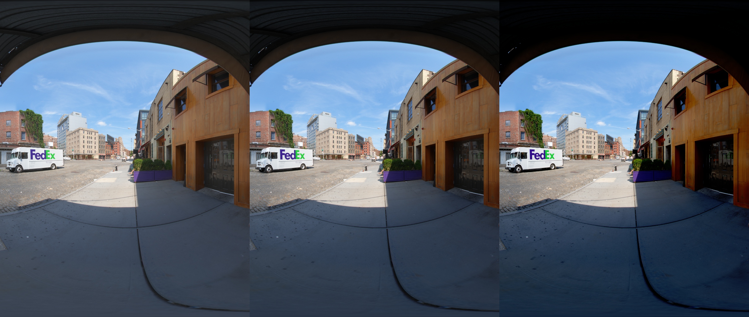
Example Images
Here are a few comparison images. The source image is a crop of the “Wooden Door” from Christian Bloch’s sIBL Archive.
First, here is an example of an on/off comparison of the filmic curve to linear.
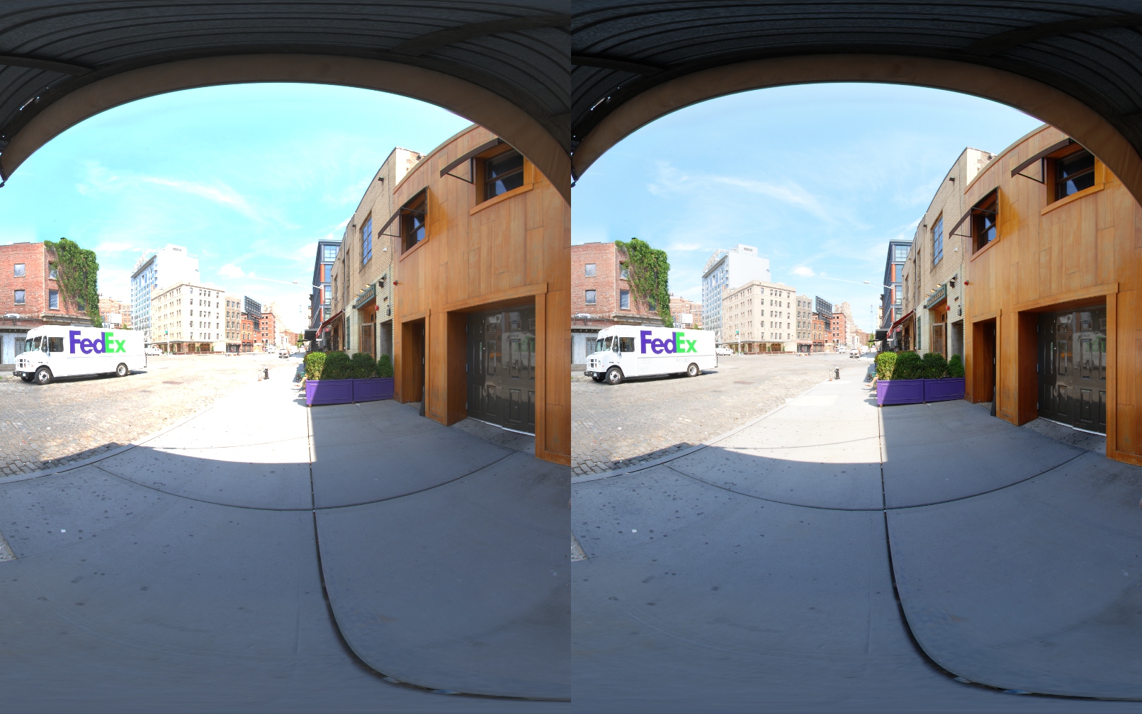
Linear vs Filmic
In this image, the filmic curve is applied with no shoulder on the left to a full shoulder on the right. It brings the highlights back into range. The shoulder parameters have no effect on the toe, so the shadows are unchanged.
Shoulder
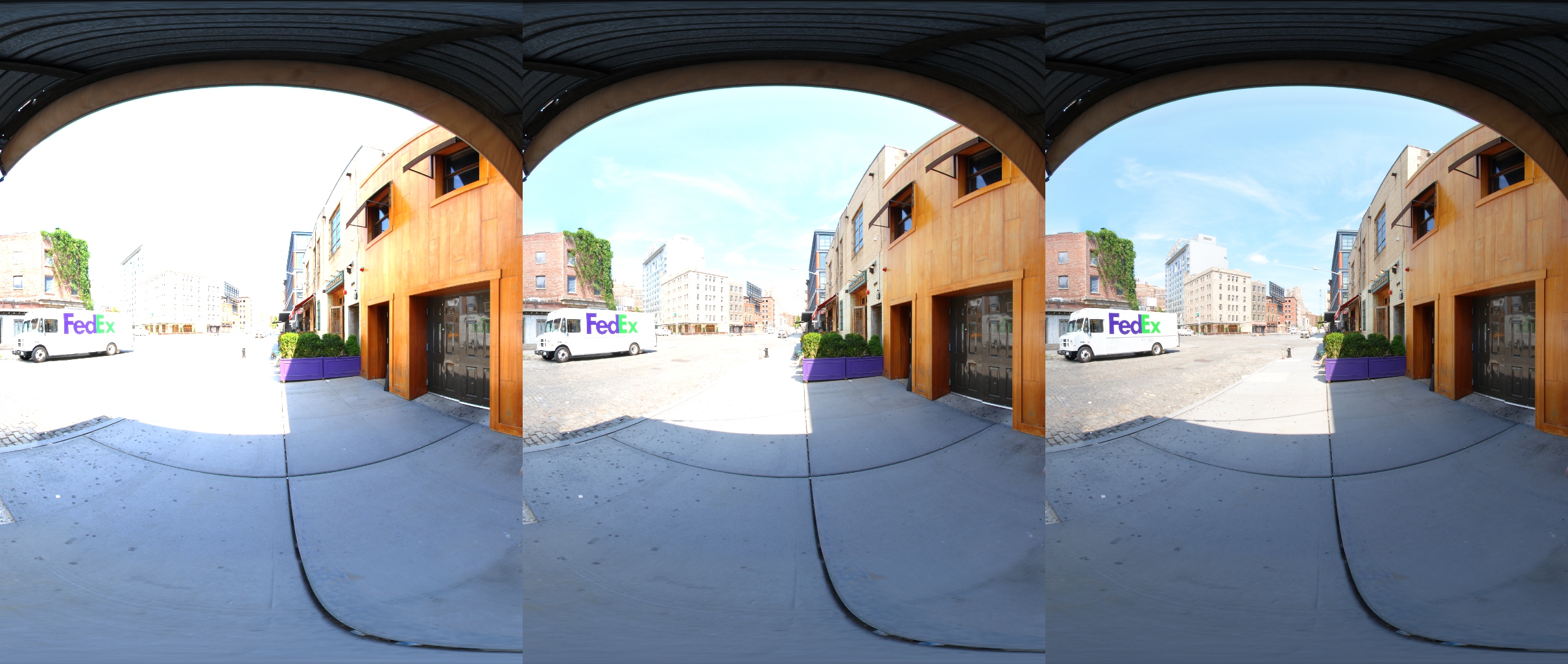
This next image shows the effect of overshoot. Without overshoot, the image on the left looks too cyan-ish because while the green and red channels are not clamping they are getting too close to 1.0. Whereas the image on the right with overshoot enabled preserves detail in the overexposed areas. There is also more detail in the sidewalk in the sunlight.
Overshoot
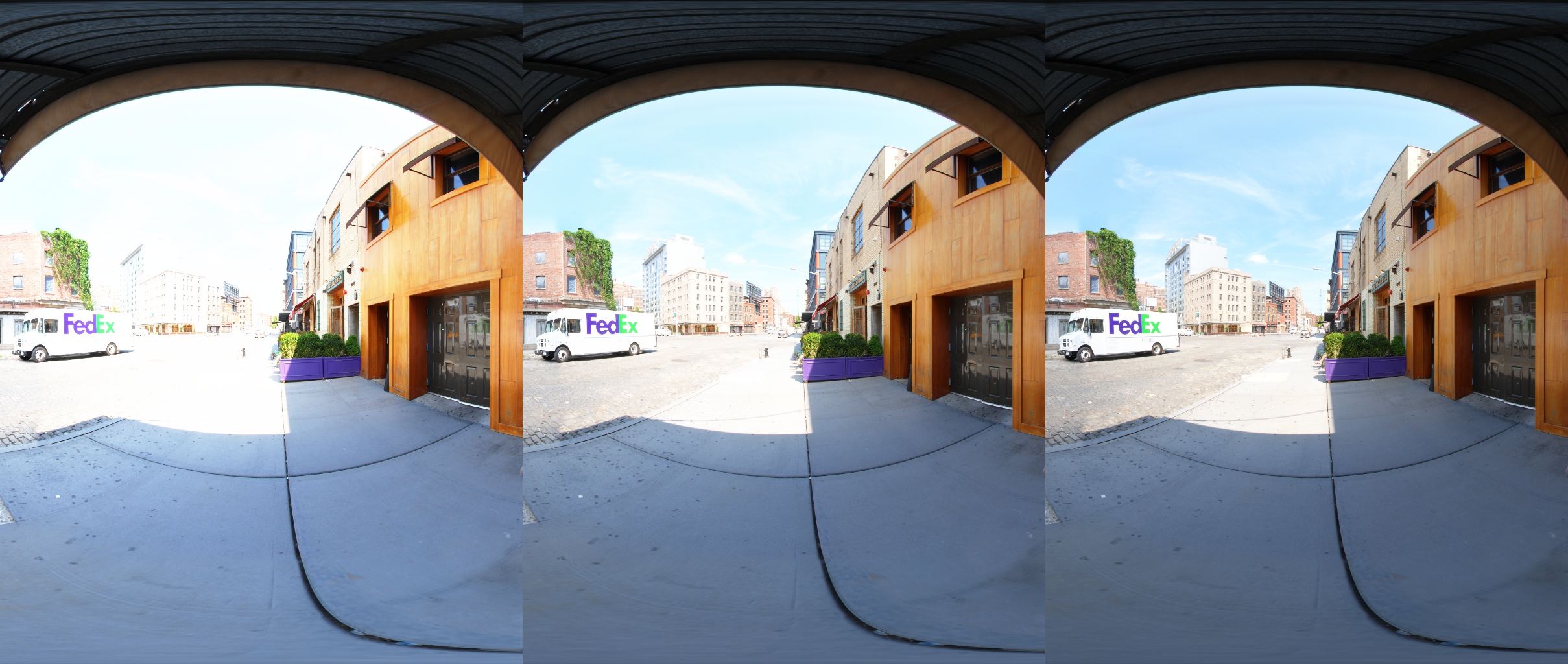
And here is an example of the toe strength param. Notice how it brings down the blacks but leaves the highlights mostly alone. Changing the toe does change the rest of the curve, but these changes are minimal.
Toe
Default Linear Params
How these parameters are set up in the engine is up to the developer. I prefer to set the toeStrength and shoulderStrength to 0 with toeLength and shoulderLength set to reasonable values for tweaking (like 0.5). That way the default curve is actually linear, and the strength parameters define how nonlinear you want the filmic curve to be.
Some people disagree with me on that. The argument goes “If the user enables Filmic Tonemapping, then the user should immediately see something happen.” I understand that argument, but I disagree for game teams. Your artists should understand how the filmic curve affects the final scene, and the best way to help them learn is to always start with linear and add as much range as you need.
Starting with linear has the side benefit of making the transition easier. If your game is currently linear, you can turn on the filmic curve and nothing happens. Then you can add more toe and shoulder gradually as needed. To me, this transition plan is preferable to having a major change to the “look” of your game that you have to fix all over the place on a case-by-case basis. Honestly, I don’t really care if your default parameters have a strong affect or if they are a no-op, but my preference is to start as linear.
That being said, if you need some default parameters the following should work as a starting point for tweaking:
toeStrength = .5
toeLength = .5
shoulderStrength = 2.0
shoulderLength = 0.5
shoulderAngle = 1.0
Luminance Only
Finally, another common change I see is to apply the filmic curve to luminance only. I disagree with this practice, but there are good reasons to do it. The filmic curve will add saturation to your shadows and remove saturation from your highlights. It is an open question whether this behavior is a bug or a feature.
The simplest way to handle luminance only is along the lines of:
float3 val = ...
float srcLum = dot(val,float3(1,1,1)/3.0)
float dstLum = Tonemap(srcLum)
return val * (dstLum/srcLum);
In other words, calculate the source luminance, apply tonemap to find the destination luminance, and mulitply by the ratio. Some people prefer it, but I prefer to apply the tonemap curve to each channel manually.
As a theoretical example, let’s say that you have a tonecurve that makes that following transformation:
F(0) = 0.00
F(2) = 0.80
F(4) = 0.95
F(5) = 1.00
Suppose you have an RGB value of (0,2,4) and apply the previous filmic curve to the luminance. Your average luminance which is 2.0, which gives you a tonemapped luminance of 0.8.
When you apply that scale (0.8/2.0) to your initial color (R=0,G=2,B=4) you end up with (R=0,G=.8,B=1.6). Even though your input blue value was 4.0, and the white point is 5.0, your blue value will still clamp. The fundamental issue is that linear operations do not behave nicely after applying an S shaped curve.
Taking this to an extreme, suppose that we were instead processing the color (R=4,G=4,B=4) with the same tone curve. Our average luminance is 4.0, which tonemaps to, say, 0.95. Then we apply that scale (0.95/4.0) to our initial color (R=4,G=4,B=4), and we end up with (R=0.95,G=0.95,B=.95).
In this test case, the blue value of (R=4,G=4,B=4) is actually lower than the blue value of (R=0,G=2,B=4) due to crosstalk between the channels. We end up with this weird situation where blue is clamping because there is not enough red. This happens because preserving the hue and saturation of a color after applying a filmic S curve is not well defined.
However if we had applied the filmic curve to each channel individually, we would have a value of (R=0,G=0.8,B=0.95) which preserves detail in the highlights. As we get closer to white, we WANT to reduce the saturation. A tone cuve that gradually removes saturation from highlights as they become overexposed is a feature, not a bug (IMO).
That being said, it is personal preference. We are dealing with artistic choices so there is no correct answer. But for the record, my preference is to apply the filmic curve to each channel separately.
Github
Here is source code on github. Also on there is the source code for my next post, Minimal Color Grading Tools.
github.com/johnhable/fw-public
comments powered by Disqus